 In appeared the question: How can I explain the dimension idea, without step in a hard topology frame, but further of the Euclidean simplicity? Here is a slightly expanded version of my answer given there.
Dimension is surprisingly hard to explain on a calculus level without escaping to topology or measure theory. Related is the concept of a boundary which appears also not to be easy to grasp. The concept of boundary turned out to be one of the more difficult problems in a recent final exam [PDF].
A generic answer
In calculus, a geometric space X in 
")


Dimension is best explained at first with concrete examples: isolated points have dimension 0, curves like a line or circle have dimension 1, surfaces like the unit sphere in 3-space have dimension 2, solids like solid balls in Euclidean 3-space have dimension 3. It can surprise at first that the solution set to a single equation can lead to different dimensions: 


 = \langle u+v,u+v,u+v \rangle")

,r sin(t), r \rangle")

Hausdorff dimension
The Hausdorff dimension requires some real analysis background. It is a dimension for metric spaces and not a topological invariant as it can change under homeomorphisms. One can push it into intro classes like Handout for Math21b, 2004, Handout from Math 118r, 2005. One first defines the (s,r)-volume as the infimum over all 

/log(r)")


/\log(r) = \log(20/log(3)")

/\log(3)")
A worksheet with some examples is here [PDF].
Hausdorff-Uhryson dimension
The Hausdorff-Uhryson dimension is a topological notion but it is integer valued. Start with =-1")


Inductive graph dimension
A finite simple graph G=(V,E) is simple geometric structure, but it becomes mighty if equipped with more structure like dimension, homotopy or simplicial complexes. A subset W of the vertex set V defines a subgraph H=(W,F), where F is the set of edges (a,b) with both a,b in W. This graph is called the graph generated by W. The graph generated by the unit sphere of a vertex x (the set of vertices directly connected to x), is denoted S(x). As there are in general no unique geodesics in a graph, graph geometry is essentially a sphere geometry. And there is hardly anything in the continuum which can not be done in graphs. Motivated by the inductive Menger-Uryson dimension, one can define:
| The dimension for a finite simple graph is defined as 1 plus the average of the dimension of the unit spheres S(x). The dimension of the empty graph is -1. |
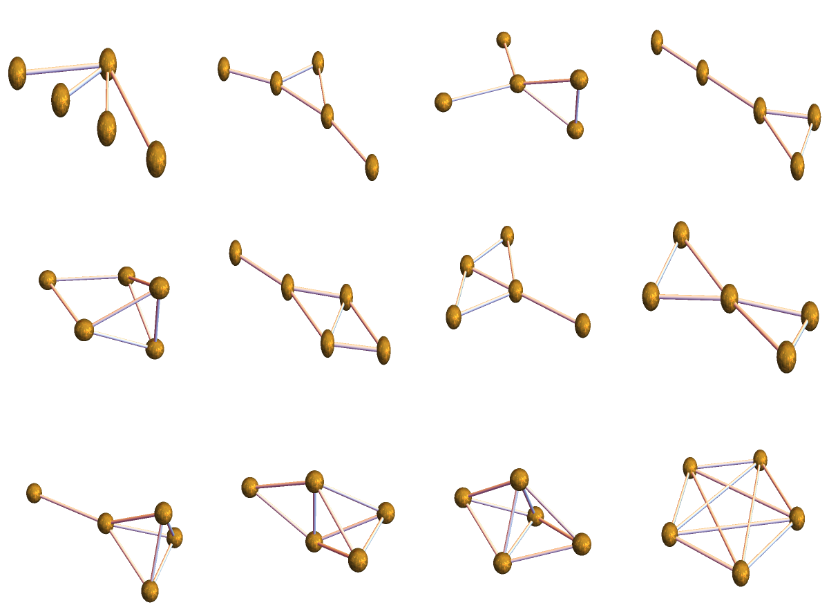
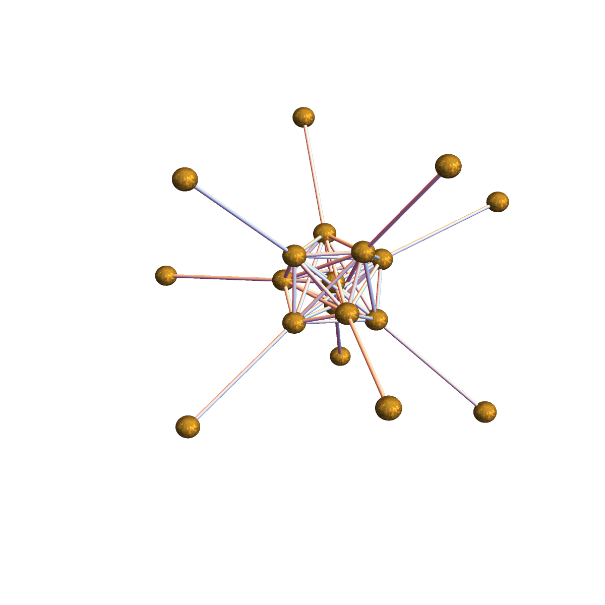
The dimension functional takes 12 different values on the set of 728 connected graphs with 5 vertices. Here are the 12 representatives again. (It is a figure given in this article). The inductive dimensions of the graphs in this figure are 1,4/3,7/5,22/15,23/15,5/3,17/10,2,49/20,79/30,3 and 4. The dimension functional on graphs with n vertices takes dimension between 0 and n-1.
Four dimensional space
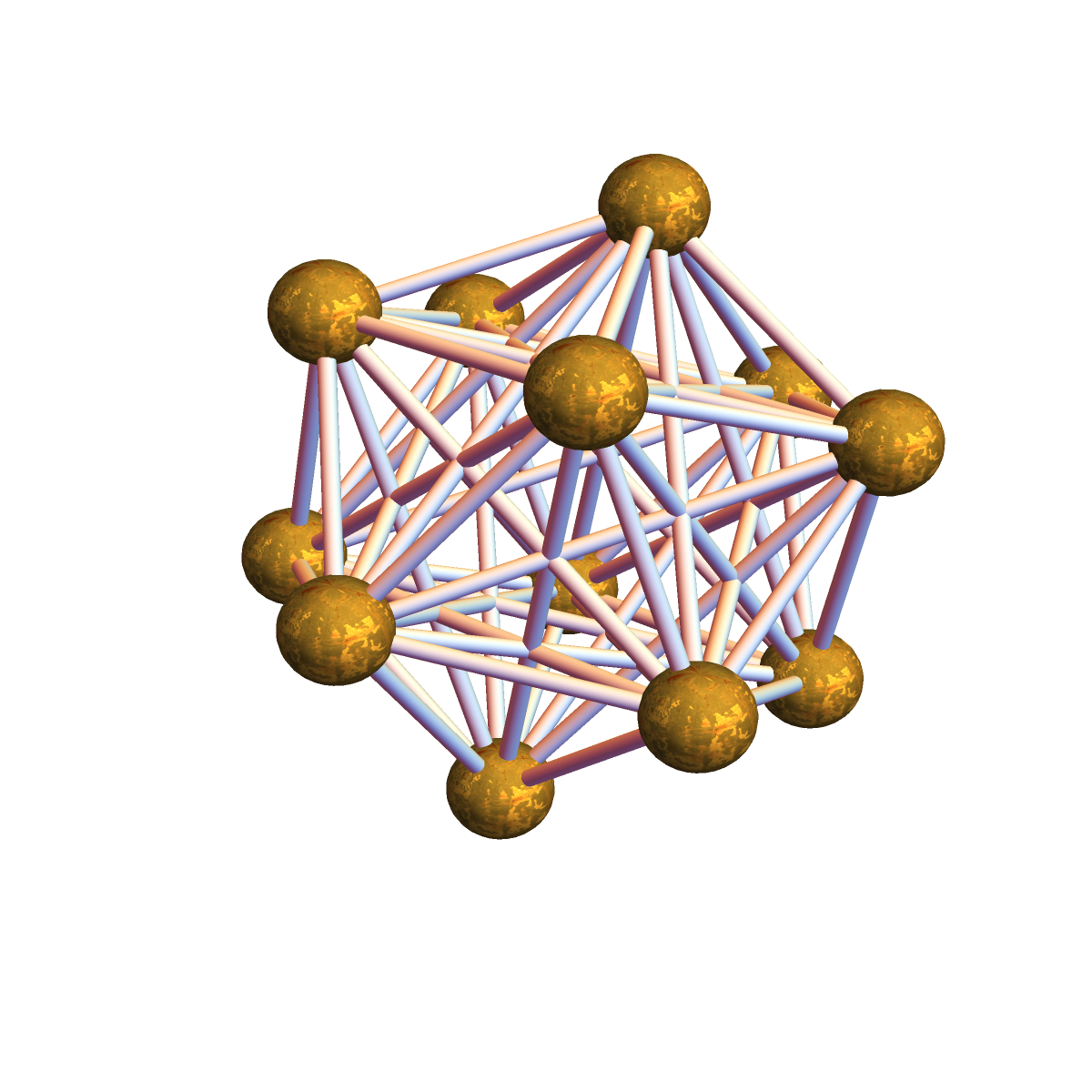
A picture of a 4-dimensional space can be obtained by drawing 5 points and connect all with each other. This defines a 4-dimensional simplex. Why is it four dimensional? Because all unit spheres are 3 dimensional simplices (tetrahedra=K4). Why is a tetrahedron 3-dimensional? Because all its unit spheres are triangles (two dimensional). Why is a triangle two dimensional? Because all its unit spheres are intervals. Why is an interval one-dimensional. Because all its unit spheres are isolated points. Why is an isolated point zero dimensional? Because all its unit spheres are empty.
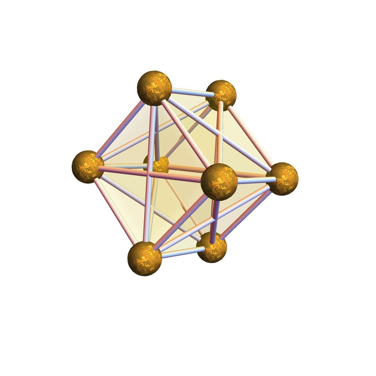
Now lets look at a visualisation of the three-dimensional sphere. We don’t mean the 2-sphere bounding the three dimensional ball but the 3-sphere, which is a three dimensional space usually thought of as embedded in a four dimensional space and realized for example as x2 + y2 + z2 + w2=1 or as the set of unit quaternions. In the discrete, the simplest 3-sphere is the 4-cross polytop. It has 8 vertices. We can realize that sphere nicely by drawing 6 vertices on a circle and two inside. On the circle, connect all except opposite ones. Now connect all two inner vertices with all the vertices on the circle. A better picture is to let the vertices be the corners of a cube. Now connect along the edges of the cube and along the diagonals. Why is the cross polytop with 8 vertices a three dimensional sphere? The reason is that removing one vertex renders it contractible and because every unit sphere in that graph is an octahedron graph. Why is an octahedron graph a two dimensional sphere? Because removing one vertex produces a wheel graph, which is contractible, and because every unit sphere is a circular graph C4 which is a one-dimensional sphere. Why is a C4 graph a one-dimensional sphere? Because removing one vertex renders it contractible and because every unit sphere is a 2 point graph without edges (which is a 0-sphere). Why is the later a 0-sphere? Because removing one vertex renders it contractible (it is a single point) and because every unit sphere is the empty graph (a (-1)-dimensional sphere. The f-vector of the 3-sphere is (8, 24, 32, 16) meaning that there are 8 vertices, 24 edges, 32 triangles and 16 tetrahedra (complete graphs K4) in this graph. The Euler characteristic is the “super sum”, which is 8-24+32-16 = 0. Its not only that 3-spheres always have Euler characteristic 0, every 3 dimensional discrete manifold (a graph for which every unit sphere is a graph theoretical 2-sphere) has this property. There is a general Gauss-Bonnet-Chern theorem for graphs. The curvature of the 3-sphere is constant 0 everywhere. This turns out to be true in general for any 3 dimensional geometric graph. This is proven here using probabilistic methods: the curvature is the expectation of Poincare-Hopf indices. It turns out that one can see this zero curvature result also as a special case of the Dehn-Sommerville relations extended here to multi-linear valuations.
Product and expectation
There are two reasons why the inductive dimension for graphs is natural: 1. It satisfies the dimension inequality  \geq dim(G) + dim(H)")
The inductive graph dimension for graphs is not the same than the inductive Menger-Uryson for metric spaces, as the later assigns always the dimension 0 to graphs (natural finite topological spaces on graphs are usually discrete topologies). The inductive dimension is well suited for simplicial complexes in the sense that one can prove nice theorems. The case of abstract finite simplicial complexes is a bit more general: define the dimension of a point $x$ in a simplex abstractly as 1 plus the dimension of the simplicial complex generated by all simplices which are sub or sup complexes of $x$. In full generality, this inductive dimension satisfies the dimension inequality  \geq dim(G) + dim(H)")
Other dimensions for graphs
In graph theory, various notions of dimension have been introduced but they are all different from the inductive definition given above (introduced in 2010 and worked out more generally in 2011). Here is a sample of definitions:
- The maximal dimension of a graph G is the dimension of the Whitney simplicial complex on G. It is the length of the $f$-vector minus $1$. The dimension of the complete graph
is
- The Erdoes-Hararay-Tutte dimension of a graph is the least k such that the graph can be embedded into Rk in such a way the Euclidean distance between two adjacent vertices is one. The complete graph Kn has dimension n-1 but a wheel graph already has dimension 3.
- The Covering dimension of a graph is the minimal k such that every open cover of $G$ has a subcover such that no point is included in more than k+1 elements in the cover.
- The Wiener dimension of a graph is the cardinality of the image of the map
. The dimension of every complete graph
- As mentioned before the small inductive dimension of a graph is $0$.
Abstract manifold notions in metric spaces
Define an abstract d-manifold as a compact metric space (X,d) for which small enough unit spheres are abstract (d-1) spheres, An abstract d-sphere is a d-manifold which when punctured becomes contractible in some homotopy sense. The notion of homotopy also goes over abstractly to discrete cases by defining it inductively: a homotopy step either adds a point to a contractible set or removes a point with contractible sphere. [On graphs, this leads to Evako homotopy and Evako spheres.The Evako homotopy has essentially been introduced by Whitehead but as far as we can see, before Evako, one always referred to Euclidean realizations. Staying completely and maybe Brouwer fanatically in the discrete so by rejecting the notion of infinity has advantages in that one stays close to computer science. ] On general metric spaces, the notion of d-manifold will depend on the chosen notion of homotopy. The local r-dimension at a point x can then be defined as )")
")
Inductive dimension in metric spaces
Here is an inductive dimension in metric spaces:
| The empty set is a metric space with dimension -1. A metric space (X,d) has dimension k if every small enough sphere S(x) with induced metric is a metric space of dimension k-1. |
An isolated point has dimension 0 because sufficiently small spheres have dimension -1. A curve has dimension 1 since if we take a point x on this curve and look at all the points in a small distance r from x, this is a discrete point set of dimension zero. A surface like the sphere is two dimensional because if we pick a point, and draw with a ruler the set of points with fixed distance from this point, then we get for small nonzero r a circle which we have already established as having dimension 1.
A probabilistic generalization
More general is a metric space equipped with a nice enough probability measure which we call inductively “nice” if it induces nice measures on small enough r-spheres. Now we say $x$ has dimension k if ")


| The empty set is a metric space X with r-dimension -1 equipped with a probability measure. Assume the metric is rescaled so that diameter of X is 1. The local r-dimension dim(x) of X at x is the 1 plus the dimension of Sr(x). Inductively we always assume the new metric on spheres is rescaled so that the diameter is 1. The r-dimension of X is the expectation value of r-dimension random variable dim(x). |
Examples:
- For compact Riemannian manifolds and small enough r, the volume probability measure is a nice measure. It induces nice measures on geodesic spheres, which are again nice Riemannian manifolds equipped with a nice measure. As mentioned, we rescale the metric on each sphere
- For a finite simple graph and r=1, we get the inductive dimension defined above.
Is there a dimension inequality for r-dimension? Can one show that the Hausdorff dimension can be obtained as a limiting case, possibly averaging over small r and taking a limit? This would link inductive and Hausdorff dimension on a general level and especially reprove the above dimension inequality. In any case, dimension and homotopy together can characterize Euclidean spaces or locally Euclidean spaces like manifolds. But it is more general.
Topological notions in graphs
In this paper a notion of homeomorphism is introduced for graphs which seems to work well. It uses homotopy and dimension. It is defined in such a way that cyclic graphs