To this article:
There are various cohomologies for finite simplicial complexes. If the complex is the Whitney complex of a finite simple graph then many major results from Riemannian manifolds have discrete analogues. Simplicial cohomology has been constructed by Poincaré already for simplicial complexes. Since the Barycentric refinement of any abstract finite simplicial complex is always the Whitney complex of a finite simple graph, there is no loss of generality to study graphs instead of abstract simplicial complexes. This has many advantages, one of them is that graphs are intuitive, an other is that the data structure of graphs exists already in all higher order programming languages. A few lines of computer algebra system allow so to compute all cohomology groups. The matrices involved can however become large, so that alternative cohomologies are desired.
A second cohomology is Cech cohomology. It is defined once one has defined a notion of topology and so of a nerve graph of an open cover. Cech cohomology leads in general to much smaller matrices which makes the computations easier. But the construction of the nerve graph is not canonical. About the notion of a topological structure on the graph: Homeomorphisms defined in traditional topological graph theory assume the graph to be a one-dimensional simplicial complex. Graphs however, when equipped with the Whitney complex, are full grown-up geometric spaces for which many results from the continuum generalize. A notion of topology for such general graphs allows to define what a homeomorphism is. It also allows to define a Cech cover. See this article.
A third cohomology is de Rham cohomology. For de Rham cohomology, one first has to have a good notion of graph product, otherwise, it is not defined. There is indeed a natural topology which makes things work nicely. There is then a discrete de Rham theorem showing that the cohomologies are the same. Also de Rham cohomology leads in general to much smaller matrices, but it assumes that the graph is a product of other graphs or then patched together with different charts which are made of products. See the Kuenneth paper.
We recently stumbled upon a fourth cohomology for graphs: Morse cohomology. It has become a fancy cohomology in dynamical systems theory, especially after it got enhanced by Floer to prove the Arnold conjectures. The story in the continuum is quite well established with Thom, Milnor, Smale, Witten etc. We have not yet explored it in full generality, but here is what has been shown already (see this paper, [January 25, now on ArXiv]).
Theorem: given a finite simple graph G=(V,E). There exists a Morse function f:V1 -> R on the vertex set V1 of the Barycentric refinement G1 = (V1,E1) of G for which the Morse cohomology is defined and equivalent to simplicial cohomology.
What still has to be done is to identify a general class of Morse-Smale functions for which the Morse cohomology works and is equivalent to the simplicial cohomology. Here is proof: there is a natural Morse function on the Barycentric refinement: it is the function f(x) = dim(x), the dimension of the point x, when it was a simplex in the original graph (remember that in the Barycentric refinement G1 the vertices were the simplices in G). It is locally injective (aka a coloring) by definition and a Morse function in the sense that the graph S–f(x) generated by all vertices y in the unit sphere S(x) of a vertex x for which f(y)
For the function f=dim, every point is a critical point. The Morse index of a critical point is defined to be equal to m, if the sphere S–f(x) has dimension m-1. Actually, when adding the point x to the graph f(y)< f(x), a m-dimensional handle (m-ball) has been added. Its boundary is the sphere. The chain complex X for Morse cohomology are functions on critical points, graded by the Morse index. We have X= X1 + …. + Xm. So, 0-forms are functions on vertices of Morse index 0, 1-forms are functions on vertices of Morse index 1 etc For Morse cohomology, one defines an exterior derivative d: Xm -> Xm+1 given by df(x) = sumy n(x,y) f(y), where x is a point of Morse index m+1 and the sum is over critical points of Morse index m. The number n(x,y) is the intersection number of the stable manifold of x and the unstable manifold of y. The difficulty to make this general is that one has to be able to define stable and unstable manifolds as well as to have a reasonable intersection number.
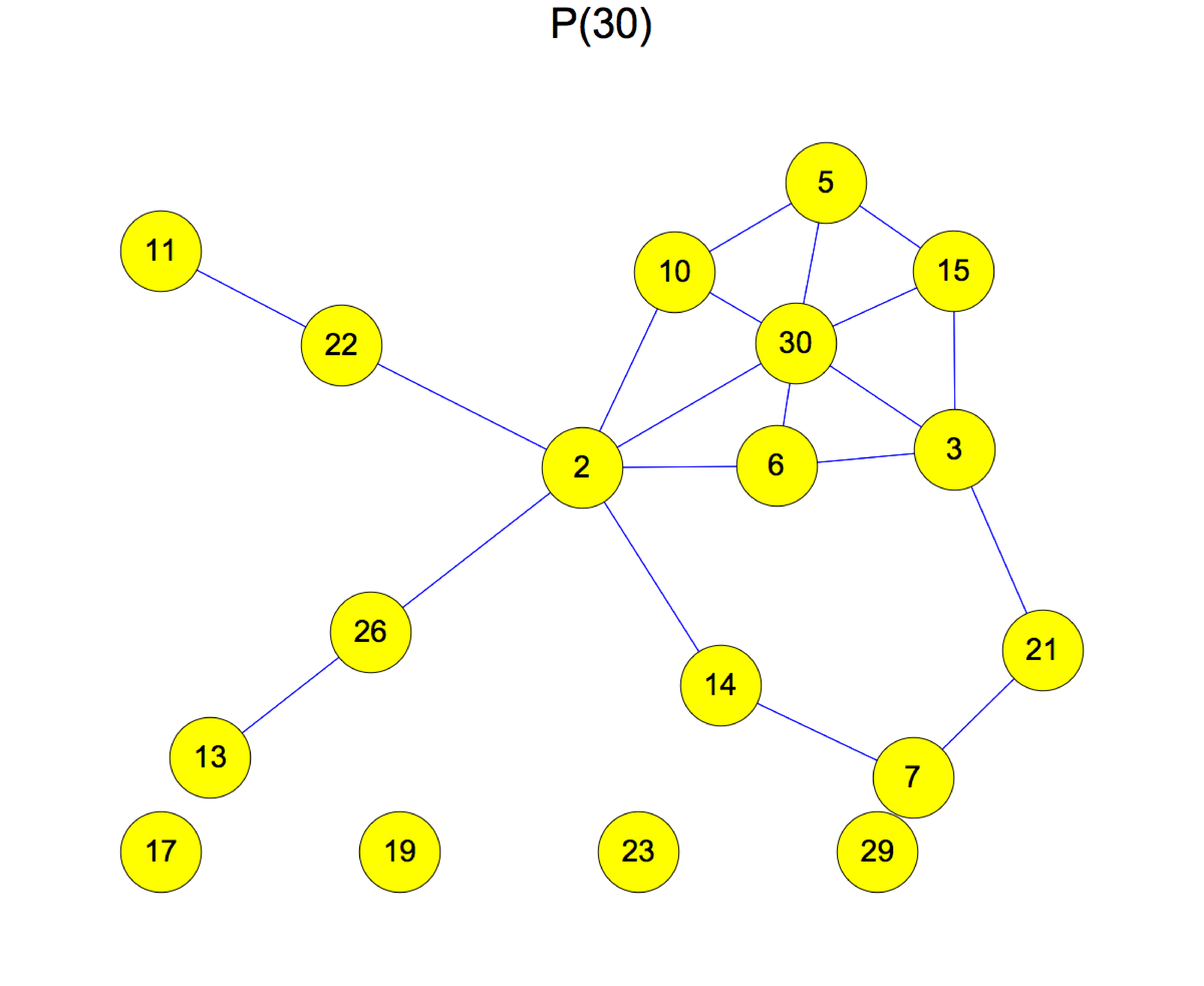
Where does counting come in? We can for each integer n define a graph G(n) for which the vertices are the square free integers in the interval [2,n] and where two integers are connected, if one is contained in the other. Here is the graph G(30). What just happened when adding the number 30, is that a two dimensional handle (disc) has been added to the graph. It destroyed a one-dimensional circle and changed the first Betti number of the graph. It turns out that during counting, the topology of the graph G(n) does not change when adding an integer for which the Moebius function is zero. Actually, the Moebius function of a vertex x is a minus the Poincaré-Hopf index of x. And The Euler characteristic X(G(n)) is equal to 1-M(n), where M(n) is the Mertens function. In the case n=30 for example, we have mu(30)=mu(3*5*2) = -1 so that the index is 1. Indeed, when we added the vertex 30, the unit sphere of 30 is a 1-sphere of Euler characteristic 0 so that the index is i(30) = 1-X(S(30)) = 1. The Betti number has increased by 1 as a one dimensional hole has been filled. As described in the text (PDF), counting is a rather dramatic process, telling the story of birth and death of spheres. The example is interesting also as it is a case, where one can almost immediately see the relation between Morse cohomology and simplicial cohomology.