Code for QR inflation - Quantum Calculus

Here is again some Mathematica code. What is new here, that we do not bother to solve the Lax differential equations but directly compute the deformation using QR which is exact. We build a small 3 sphere as a simplicial complex G, then build the Dirac matrix B=D (we chose the letter B because D is used in Mathematica for derivatives). Then we chose a small h so that h B has norm smaller than 1 and so that the theorem applies with g(B)=-log(1+h B) so that the isospectral deformation of $(1+h B)^t = Q_t R_t$ gives the unitary $Q_t$ , deforming B to $B_t=Q_t^* B Q_t$ , which now is of the form $c_t + c_t^* + m$ , with electromagnetic part $C=c+c^*$ and diagonal dark matter part $m$ . The size of the electromagnetic Laplacian c is then computed which is inversely proportional to the Connes diameter of the space. We see that the space initially starts to inflate fast and then slows down to a more or less constant rate of expansion. This is a mathematical phenomenon and has nothing to do (a priori at least)with any “cosmic inflation” one sees in the early universe. Cosmologists seem to have no clue what has driven the cosmic inflation. One can read about a “hypothetical scalar field” or about “false vacuum” which indicates that one has no idea. As for what is known, the consensus seems that there must have been a period of fast expansion. We also have strong evidence that space itself expands.

What we see here is just a mathematical phenomenon which holds for any geometry, any space with an exterior derivative. It can be a random network. If you experiment, make sure that t is an integer (discrete time). Mathematica not so elegantly can segfault if one gives a real argument t to MatrixPower[A,t]. Also larger t makes ,the code unstable because we take large matrix powers and then make a QR decomposition of such a large matrix. What is new (as pointed out last week) is that we have illustrated the already in the paper of 2024 written remark that with this choice of g(t) in the deformation, the Q_t is causal. Mathematically, this means that Q_t is a Jacobi type matrix in a strip where the width of the strip is not wider than t. This comes from the fact that a time step is a a cellular automaton map, only affecting the effective neighborhood of the simplicial complex. We had for philosphical reasons insisted on that. We want a causal evolution. Something at the other end of the simplicial complex should not immediately affect the situation at the other end. Signals should need time to propagate. Mathematically this means that $u(t) = Q_t u(0)$ should have support roughly in a t -neighborhood of x if u(0) was initially supported on x.

Generate[A_]:=If[A=={},{},Sort[Delete[Union[Sort[Flatten[Map[Subsets,A],1]]],1]]];
Whitney[s_]:=Union[Sort[Map[Sort,Generate[FindClique[s,Infinity,All]]]]]; L=Length;
sig[x_]:=Signature[x];   nu[A_]:=If[A=={},0,L[A]-MatrixRank[A]];  omega[x_]:=(-1)^(L[x]-1);
F[G_]:=Module[{l=Map[L,G]},If[G=={},{},Table[Sum[If[l[[j]]==k,1,0],{j,L[l]}],{k,Max[l]}]]];
sig[x_,y_]:=If[SubsetQ[x,y]&&(L[x]==L[y]+1),sig[Prepend[y,Complement[x,y][[1]]]]*sig[x],0];
LowerT[A_]:=Table[If[i>=j,0,A[[i,j]]],{i,Length[A]},{j,Length[A[[1]]]}];          h=0.001;
Dirac[G_]:=Module[{f=F[G],b,d,n=L[G]},b=Prepend[Table[Sum[f[[l]],{l,k}],{k,L[f]}],0];
   d=Table[sig[G[[i]],G[[j]]],{i,n},{j,n}];{d+Transpose[d],b}];   T=Transpose; CO=Conjugate;
QR[A_]:=Module[{FF,B,n},FF=T[A];n[x_]:=x/Sqrt[x.CO[x]]; B={n[FF[[1]]]}; Do[v=FF[[k]];  
   u=v-Sum[(v.CO[B[[j]]])*B[[j]],{j,k-1}];B=Append[B,n[u]],{k,2,L[FF]}];{T[B],B.CO[A]}];
QR[B_,t_]:=Module[{Q,R},{Q,R}=QR[MatrixPower[IdentityMatrix[L[B]]+h*B,t]];Chop[T[CO[Q]].B.Q]];
ElectroMagnetic[A_]:=Module[{d,e,m},d=LowerT[A];Tr[CO[T[d]].d]];
s=CompleteGraph[{2,2,2,2}]; G=Whitney[s];{B,b}=Simplify[Dirac[G]];
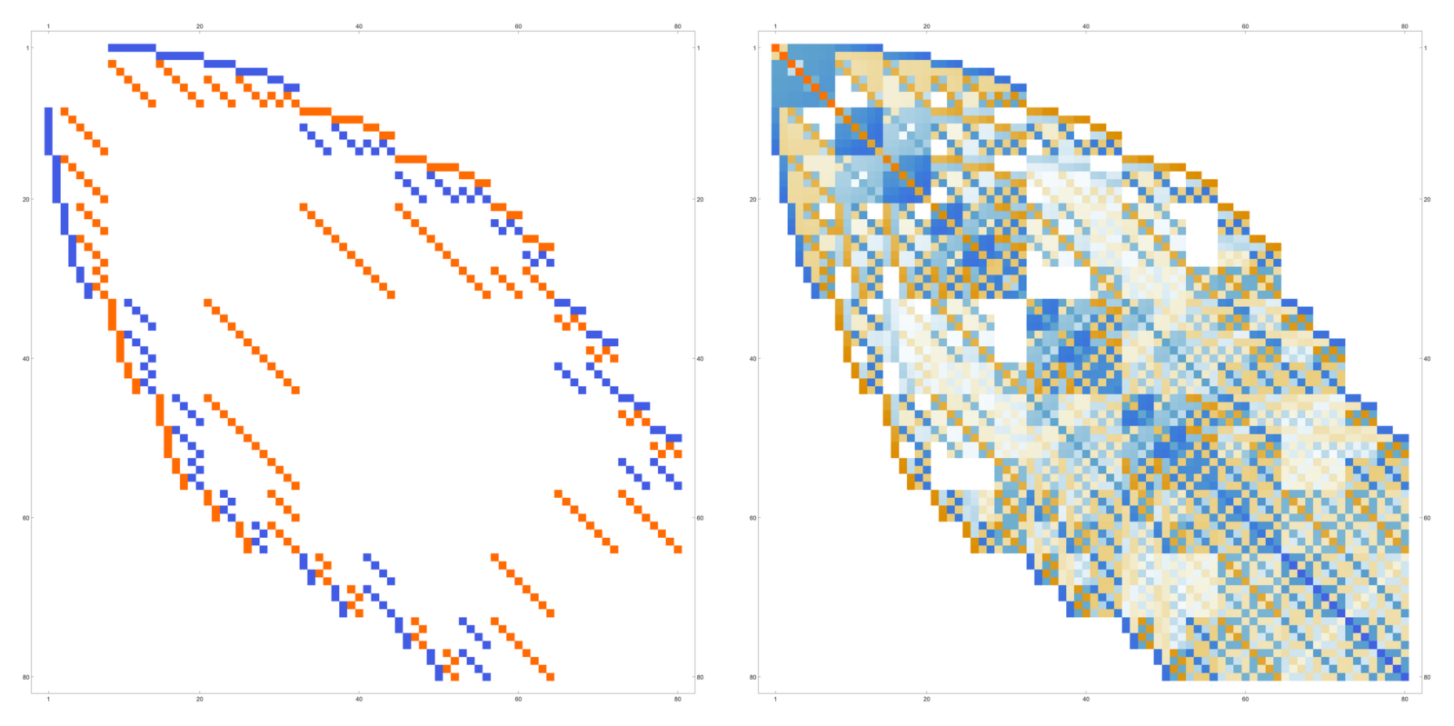
GraphicsRow[{MatrixPlot[QR[B,0]],MatrixPlot[QR[B,200]]}]
ListPlot[Table[(ElectroMagnetic[QR[B,t]]-ElectroMagnetic[QR[B,t-1]])/h,{t,0,2000,5}]]

And here is the output. We see first the Dirac matrix at t=0 then at t=200 (where a diagonal part has developed). The two matrices are isospectral. Then we see the derivative of the norm of c(t) as a function of time to t=2000. The electromagnetic part c(t) is an exterior derivative at all times producing the same cohomology but first decaying fast reaching a maximal decay rate then slowing down to an expansion rate close to 0. This is like in a logistic situation. Initially a lot of the initial exterior derivative is fueled into the dark matter part, which eventually gets saturated. In the limit the Dirac matrix is diagonal containing the eigenvalues. In that t=infinity case we would no more have any cohomology of course. To experiment, change the graph s to any network like s = RandomGraph[{15, 60}] The matrices are then already 500 x 500 matrices in general, the computation of the second graph will now take time.

Author: oliverknill