Standard Map Game

The topic is a combination of the “particles and primes” and geodesics in discrete manifolds” topics, I had worked on before. The first one is an elementary connection between primes in division algebras and particle phenomenology, the second is a completely deterministic dynamical system in combinatorics that has many properties of the geodesic flow in the continuum. The first topic goes more into number theory, the second one goes more into differential geometry, as the notion of geodesic is crucial for defining notions like sectional curvature. Both topics are related to theorems in classical mathematics. Division algebras are chosen because associative division algebras have only two examples, similarly as the standard model. As rings they have natural maximal orders and a natural number theory like almost unique prime factorization. The combinatorics of the primes have shown affinity with the particles we observe in the standard model.

First some remarks

The topic covered here is also linked naturally because it is at the intersection of two famous crackpot indices: the one for physics and the one for number theory. Maybe just go directly to the code and run the simulation and try to understand what the game does before shelving the topic as such. Mathematicians also tend to dismiss elementary parts as “trivial”. A better word for “trivial” is “elementary”. The number theory of primes is elementary but highly non-trivial, the geodesic flow on even simple geometries is elementary but highly non-trivial too. There are reasons why the subject of fundamental physics and the subject of elementary number theory are both so popular and attractive: the questions are simple and beautiful: what are the fundamental laws of the stuff we are made of? What are the secrets of the primes which build up numbers? Wouldn’t it be nice if the two things were related? As mathematicians we are not really so concerned about how complex something is nor are we interested at first whether something is relevant. What is already nice is to take some structures and play with them like a child does with toys. We have plenty of toys to play with in mathematics. And it is much cheaper because we do not need a lab. Especially fun (for me at least) are toys where some things happen and where we can experiment. Physicists have their toys like the LHC, LIGO or the Webb but these are exclusive “club membership places” which only the richest (or heavily funded) can participate. Math is much more accessible. We can easily build our own toys and play with them. Here is such a toy. It might sound silly or arrogant, but we still know very little about fundamental processes. Assume for example that we just have two electrons in the entire universe. Assume they are close together and fixed. We know they repel each other with a 1/r force which is explained from the structure of the Green function of the Laplacian in three dimensional space. That force is not immediate however as we know from relativity. It needs time to pass from one particle to the other. Forces are “delayed” or “retarded” as one says in physics. The two static electrons exchange “virtual photons”. These are “unobservable particles that mediate the electromagnetic force between them”. Now, if you think about this, you really must cringe as it only sounds good; it does not really explain anything. From one of the comments in this video:

Another ridiculous idea used by physicists when they cannot have a real explanation. Consider the case of two electrons: How does a virtual particle know that another electron has come so close that the virtual particle should start its movements? Worse than this, the number of these virtual particles should be decided (by some weird and unknown mechanism, yet to be explained of course!), when the electron is close to a number of electrons, not just one. And yet worse than that is the case where the electron is close to a number of positive and negative charges. All in all, to me it just seems an attempt to sugar-coat the problem with some fancy stuff.

I completely share this sentiment. What is the difference between a real photon and a “virtual photon” in principle? Having a short life span is not the answer. How does a virtual particle know that it has to recombine again? How many such photons are there? In order to work, every electron must come with zillions of such virtual photons. What happens if the two electrons get further and further away? Since space is scale invariant, how do we deal with an infinite amount of such virtual photons just to keep the two electrons connected by forces so that till have to feel each other. How come the “density of these virtual photons” does not decay like 1/r^2 like for radiation? The virtual photons must somehow know where to be. And it gets worse if the electrons start to move as they now generate electromagnetic waves. Even if the magnetic field generated by the moving electron does not influence the electron itself it will indirectly as it does change the other electron and so indirectly itself. The quantum field description is already extremely complicated. And the theory does not really explain things like when talking bout “wave-particle duality”. (My own quantum mechanics teacher Klaus Hepp told us (the class) that understanding the wave-particle duality is something we have to figure out on our own.) If I look this up today, the answer to this is still schizophrenic: “particles can exhibit both particle-like or wave-like features”. If one talks about electrons as particles, they are “point like” which assumes that space is a perfect Euclidean space which is probably also just an illusion. The force between two electrons in principle can become arbitrary large if they are close enough. In a concrete system like an atom, one then neither uses the particle, nor the wave picture, one just looks at eigenvalues of an operator and describes changes of electron energy states by emission or absorption of “real photons”. The “virtual photons” do not even enter the picture there any more if the atom is just static. If you look at all these stories, they each make somehow sense but the entire thing just feels like a hac,k especially on the quantum field side, where one then just uses the first few interaction Feynman interaction diagrams and neglects infinitely many other terms. It appears that a full, non-perturbative approach of the question how two electrons behave in a universe is already very difficult.

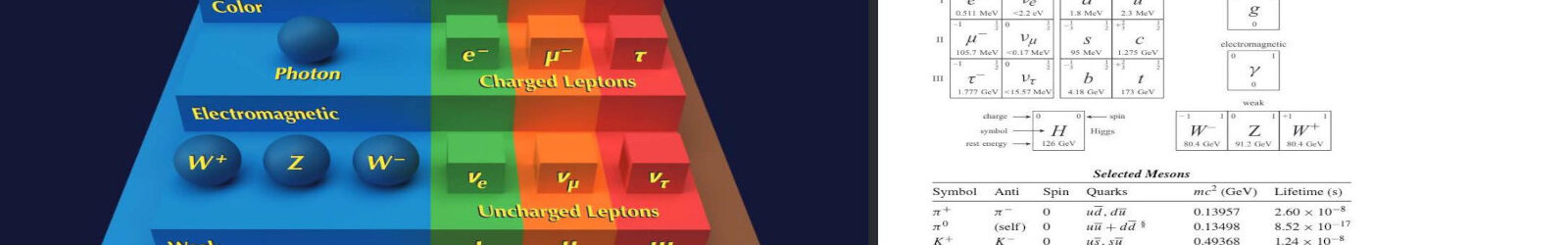
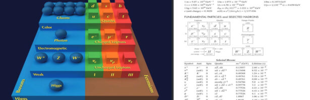
Wouldn’t it be nice if we could understand the entire game down to every detail, meaning purely combinatorially? Take a finite geometry and two electrons like 1+2i and 3+2i located at two points. Without any other particles present, they both move on geodesics. They do not know of each other. If space is filled with a sea of particle -antiparticle pairs, then the toy model has the feature that these particle anti-particle pairs do not move. The dynamics T=BA just leaves them at the same position. The map A renders the particle an anti particle and B reverses it again a particle (the original one). What happens however if an electron is present is that particle-anti-particles pairs get awaken and start to move around. If we assume they are units they are Bbosons and move with the speed of light in the cellular automaton, each on geodesics. These “virtual photons” now can reach the other electron and influence its motion. Even more, the virtual photons generated by the electron itself influence the electron itself. We expect the electron to move slower because it gets bounced around and interact with the other. Now, (and this is pure speculation of course as we have not measured it), we could think that this complicated game produces something like a repulsion and that if we take an electron-positron pair, we see them attract. And if we look at quaternion primes which model mesons or baryons, we can imagine that the now more complicated interactions produces other forces like seen in the nucleus. Now similarly as in the periodic system of elements where things stop with atomic number 118, it could be that in that standard model game only smaller primes really matter in the long term explaining in some way why there are only three lepton and quark generations. What is nice about a game like chess or the game of life (or then the game introduced here) is that we do not have to care at all whether it models conflicts or life on earth well. It is just a game after all. As long as it has precise rules, we do not do anything wrong. Yes, it might be irrelevant but as mathematicians, we do not care about that. Even the simplest toys give plenty to learn.

Some remarks about the game

Since the maximal orders in the associative division algebras and are canonical (if we want to see integer divisors (*)) and show particle Lepton and Hadron particle features, it is natural to look at division algebra valued divisors. Now there are several things to look at. Units in the algebras play the role of gauge transformations. The maximal order in the quaternion also contains numbers of the form (a,b,c,d)/2 with odd integers a,b,c,d and that would not be possible to model as particles. But the Lagrange 4 square theorem and the work of Hurwitz shows that for every rational prime p, there is a Lipschitz quaternion prime (a,b,c,d) that works. In other words, we can for any prime also find a gauge equivalent Lipschitz integer.

(*) there are other maximal orders in the complex ring . In there would be the Eisenstein integers for example but they would not produce particles. For the maximal order of quaternion Hurwitz integers, it looks at first also apepars at first that we have a problem because we can not allow half integer numbers when thinking about particles. It is however a fact that any half integer number is gauge equivalent to a Lipschitz integer (with integer entries).

I decided in the game not to evolve Gaussian and Quaternion integers separately but just only use quaternions and see the complex plane as part of the quaternions. Now, this at first appears to introduce some ambiguity. Remember that rational primes of the form 4k+3 were considered neutrini because they do not split in the completion of the reals. In the quaternions such neutrini are written as (p,0,0,0), the smallest example being (3,0,0,0), then, within the quaternion order we have the factorization (3,0,0,0) = (0,1,1,1) * (0,1,1,1) so that within the quaternions, we would see this particle as a Boson (it decomposes into an even number of particles ). A similar story happens when we look at primes of the form (a,b,0,0) which can be seen as Gaussian primes a+ib and which are electrons and so Fermions. But within the quaternions, it is gauge equivalent to a second quark and so should be considered a meson. For example (a,b,0,0)=(5,2,0,0) is gauge equivalent to (a+b,a+b,a-b,a-b)/2 = (7,7,3,3)/2. In any of these cases, we have no difficulty if we define the interaction as described just using the Legendre function. [So, unlike muttered during the saturday presentation, I at the moment think it is better to use the simpler interaction. It would also be much more costly in each case to figure out the nature of each prime in the prime factorization. The number of primes in the quaternion prime factorization does not need to know the structure of the primes. As described in the Conway-Smith theorem, there is always some ambiguity about the nature of particles if bound together similarly as in nature, but we do not get any different outcome.

Just as a side remark again (I talked about this a couple of times already and it might be a bit tiresome but it was original originally:) the particle allegory might be irrelevant but it is useful as a memnonic to remember theorems. The 4k+1 primes are Bosons because they factor into two Gaussian primes the 4k+3 primes are Ffermions. If we assign to Fermions the Jacobi symbol -1 and to Bosons the Jacobi symbol 1, then the Gauss law of quadratic reciprocity tells that two odd primes satisfy the commutation relation (p|q) = (q,p) if and only if one of them is a Boson. The allegory also includes the Christmas theorem of Fermat telling that primes of the form 4k+1 are a sum of two squares or the Lagrange four square theorem which assures that there are quaternion primes for any rational prime. The off shot is that we can completely ignore physics and make mathematics more natural. Especially intriguing are unique factorization results like the one of Hurwitz (sometimes cited in a more refined way as Conway-Smith theorem but it is essentially due to Hurwitz. Primes behave llike particles also in a non-commutative setting and there, the gauge bosons are more interesting. Changing gauge bosons around changes the nature of particles, like in a nucleus, where gluons do this job.

Something else: I mentioned during the presentation thegauge invariance of the interaction. It means however if the gauge is applied to a simplex but there is no gauge invariance of course on the phase space level, when looking at the frame bundle. Every photon (unit) contributes in the interaction and the heavier vector bosons entangled with the prime 2 (which is a boson as 2i=(1+i)^2. We have chosen to add up all particles and then do the prime factorization. The interaction uses the full ring structure and not only the multiplicative or additive structure. This makes the interaction more interesting. If we take two numbers for which we know the prime factorization and we add up these two numbers, we get a completely different prime factorization. It looks pretty random. Particle processes look pretty random. We can not predict when a particle decays, there are probabilistic descriptions available only.(We even use radioactive processes as random number generators.) Any artificial randomness in a system makes things unnatural however. One does this all the time. The entire field of statistical physics deals with that. We evolve Bolzman equations or describe finite particle systems with partial differential equations pretending that the density, velocity or mass distributions are smooth functions.

Again, as mentioned already years ago, this is a topic which is a double crackpot topic triggering both number theory and particle physics crackpot checklists, lets give the code for the game. Thats what it is for now. The example demonstrates how a single particle in a sea of particle-antiparticle pairs can generate more particles. The game of course is already interesting if we do not have interaction, and where we look at the geodesic flow or billiard in a manifold with boundary. In a finite box (we took a disk or finite manifold), the particle-antiparticle pairs generated by the single initial particle will hit the particle again and alter it. The motion will after some time look rather random. Curvature terms influence the particle. Imagine for example that the particle moves over a “hill” and that some particle anti-particle parts move around the hill faster and influence the particle later on and change its direction or speed. In a curved geometry, the radiation of a particle itself can influence its own path. Dodge this bullet!

CleanGraph[s_]:=AdjacencyGraph[AdjacencyMatrix[s]];  SEE={Method ->"SpringElectricalEmbedding"};
GraphPos[s_]:=Module[{},If[Length[VertexList[s]]<1000,GraphPlot3D[s,SEE][[1,1]],GraphPlot3D[s,SEE][[1,2,2,1]]]];
GemPlot2:=Graphics3D[{A1,A2,Table[{SurfaceColor[Hue[(XX[[k,2]]-YY[[k,2]]).(XX[[k,2]]-YY[[k,2]])/10]],
        Polygon[XX[[k,1]] /. f]},{k,Length[XX]}]}, Boxed->False, Axes->False,AspectRatio->9/16];
Generate[A_]:=If[A=={},{},Sort[Delete[Union[Sort[Flatten[Map[Subsets,Map[Sort,A]],1]]],1]]];
Whitney[s_]:=Map[Sort,Generate[FindClique[s,Infinity,All]]];     L=Length;Co=Complement;Po=Position;
Facets[G_]:=Select[G,(L[#]==Max[Map[L,G]]  ) &]; RR=RotateRight; RL=RotateLeft;  S=Sort;
Bundle[G_]:=Module[{F=Facets[G]},Flatten[Table[Permutations[F[[k]]],{k,L[F]}],1]];  Se=Select;
OpenStar[G_,x_]:=Select[G,SubsetQ[#,x]&];         Stable[G_,x_]:=Complement[OpenStar[G,x],{x}];
BndFace[s_]:=Module[{G=Whitney[s],q,W},q=Max[Map[L,G]]-1;W=Select[G,L[#]==q &];Select[W,L[Stable[G,#]]==1 &]];
IntFace[s_]:=Module[{G=Whitney[s],q,W},q=Max[Map[L,G]]-1;W=Select[G,L[#]==q &];Select[W,L[Stable[G,#]]==2 &]];
SoftWhitney[s_]:=Module[{G=Whitney[s],n,H=BndFace[s],q},q=Max[Map[L,G]]-1;Sort[Union[H,Select[G,(L[#]!=q) &]]]];
SB[s_]:=Module[{e={},G=SoftWhitney[s],H=IntFace[s],q}, Do[Do[q=Sort[Intersection[G[[k]],G[[l]]]];
  If[MemberQ[H,q]||SubsetQ[G[[l]],G[[k]]],e=Append[e,k->l]],{l,k+1,Length[G]}],{k,Length[G]}];
  CleanGraph[UndirectedGraph[Graph[e]]]]; SB[s_,n_]:=Last[NestList[SB,s,n]];
lambda[z_]:=Module[{u=Sum[z[[j]]^2,{j,Length[z]}]},If[u==0,0,LiouvilleLambda[u]]];
M[z_]:=Module[{U=Co[Stable[G,z],{S[z]}]},Table[First[Co[U[[j]],z]],{j,L[U]}]];
a[x_]:=Module[{y=x,u},u=M[Delete[x,1]];If[L[u]==1,y[[1]]=u[[1]],y[[1]]=Co[u,{x[[1]]}][[1]]];y];
b[x_]:=Module[{},z=(Sort[x] /. XX) - (Sort[x] /. YY); RL[x,lambda[z]]];
c[x_]:=Module[{},z=(Sort[x] /. XX) - (Sort[x] /. YY); RR[x,lambda[z]]];
pos[z_]:=Position[F,Sort[z]][[1,1]];
A:=Block[{},Z=Table[Y1=Y[[k,1]];Y2=Y[[k,2]];Z1=a[Y1]; y1=pos[Y1]; z1=pos[Z1]; YY[[y1,2]]-=Y2; YY[[z1,2]]+=Y2; Z1->Y2,{k,L[Y]}];
    Y=Table[X1=X[[k,1]];X2=X[[k,2]];Z1=a[X1]; x1=pos[X1]; z1=pos[Z1]; XX[[x1,2]]-=X2; XX[[z1,2]]+=X2; Z1->X2,{k,L[X]}]; X=Z;];
B:=Module[{},{X,Y}={Table[b[Y[[k,1]]]->Y[[k,2]],{k,L[Y]}],Table[c[X[[k,1]]]->X[[k,2]],{k,Length[X]}]};]; T:=Module[{}, A; B;];
s=CleanGraph[PolyhedronData["Icosahedron","Skeleton"]]; s=CleanGraph[SB[WheelGraph[6],2]];
G=Whitney[s]; F=Facets[G]; P=Bundle[G];  R:=Random[Integer,2];  ps[x_]:=x[[2]];  q=L[F[[1]]-1]; p2[x_]:=x[[2]];
Y=Table[P[[k]] -> {If[Random[] < 0.005, R, 0], 0, If[Random[] < 0.005, R, 0], 0}, {k, L[P]}];
X=Table[P[[k]] -> Y[[k, 2]] + {If[k == 1, R, 0], If[k == 1, R, 0], If[k == 1, R, 0], If[k == 1, R, 0]}, {k,L[P]}];
{XX,YY}={Table[F[[k]]->Total[Map[p2,Select[X,Sort[#[[1]]]==F[[k]] &]]],{k,Length[F]}],
         Table[F[[k]]->Total[Map[p2,Select[Y,Sort[#[[1]]]==F[[k]] &]]],{k,Length[F]}]};
GemPlot1=Module[{},v=VertexList[s];e=EdgeList[s]; rho=0.1; p=GraphPos[s]; f=Table[v[[k]] -> p[[k]], {k,Length[v]}];
   e=Sort[Table[Sort[{e[[k, 1]],e[[k, 2]]}],{k,Length[e]}]]; 
   A1=Table[{SurfaceColor[Orange,White,50], Sphere[v[[k]] /. f, rho]},   {k,Length[v]}];
   A2=Table[{SurfaceColor[Yellow,White,50], Tube[e[[k]]   /. f, rho/3]}, {k,Length[e]}];];  GemPlot1;
DynamicModule[{},Dynamic[T; GemPlot2]]