Wave interpolation - Quantum Calculus

Having talked a bit about GR (general relativity) and the SM (standard model), lets talk a bit about QM (quantum mechanics). Without any doubt, GR,SM and QM are three extremely successful pillars of modern fundamental physics. Their track record with experiments is monumental (*). We have played with simple games referring to GR and SM, there is a toy aspect of QM.

[(*) One should add that there are many other very nice theories with excellent track record like solid state physics, fluid dynamics or optics but they are not as fundamental as they are emergent from more fundamental principles. There are other attempts to fundamental physics but their track record in matching experiments is not good in comparison. As mathematicians we are safer as we can just state and prove theorems or lemmas and if the proof is convincing (especially if it is simple), no propaganda is needed to convince anybody that it is of some value. So, I think the remark done here is entertaining, even so it is something we could given (with suitable scaffolding of course) as an exercise in a linear algebra course. ]

Here is a cute little result in wave dynamics or quantum dynamics. (quantum mechanics originally has been called wave dynamics). The connection these days is often not stressed enough. The mathematics of the wave equation and the Dirac equation are very closely linked as the pair of Dirac equation $i u'= Du$ , $i u' = -Du$ is equivalent to the wave equation $u_{tt} = -D^2 u$ .). It works on any finite geometry which features a calculus like a delta set or graph or simplicial complex.

On a pedagogical note, it does not involve more math than what is taught in basic linear algebra courses like math 21b at Harvard. That course is great also because it features a decent introduction to dynamical systems and operator methods in differential equations as well as Fourier theory something more “honors type” courses mostly skip. (I made once 1 minute videos for each lecture: see the 1-minute presentation about d’Alembert here on youtube).

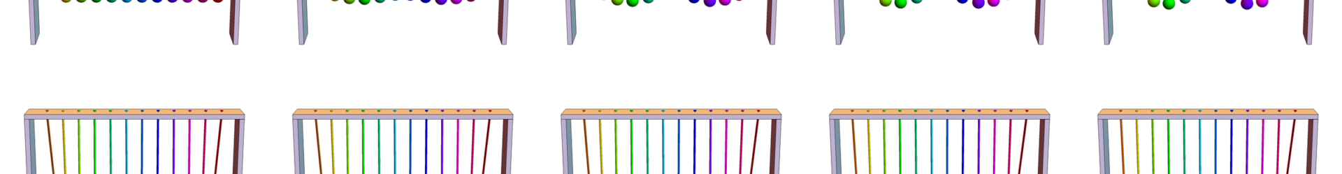
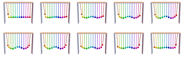
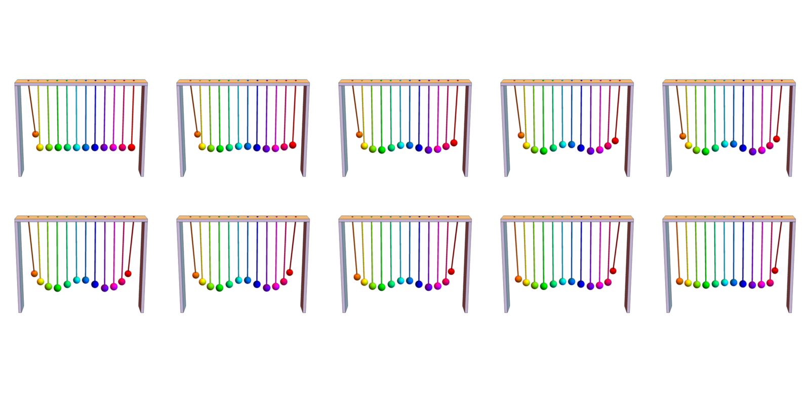
Let us illustrate the result with a picture of a row of coupled penduli (*): assume you want at time t=0 that the first pendulum is excited and no other and that at time t=1, the last pendulum is excited an no other. We can then hit all the penduli with the right amount of velocity such that the corresponding solution of the wave equation interpolates the first and second position. [ The coupled penduli I have shown in my office are a bit of a cheat as they are not really coupled. They have slightly different lengths so that the motion appears to be a wave. It is still a nice toy. I might at some point add tiny magnets on the penduli bottoms so that they get coupled. ]

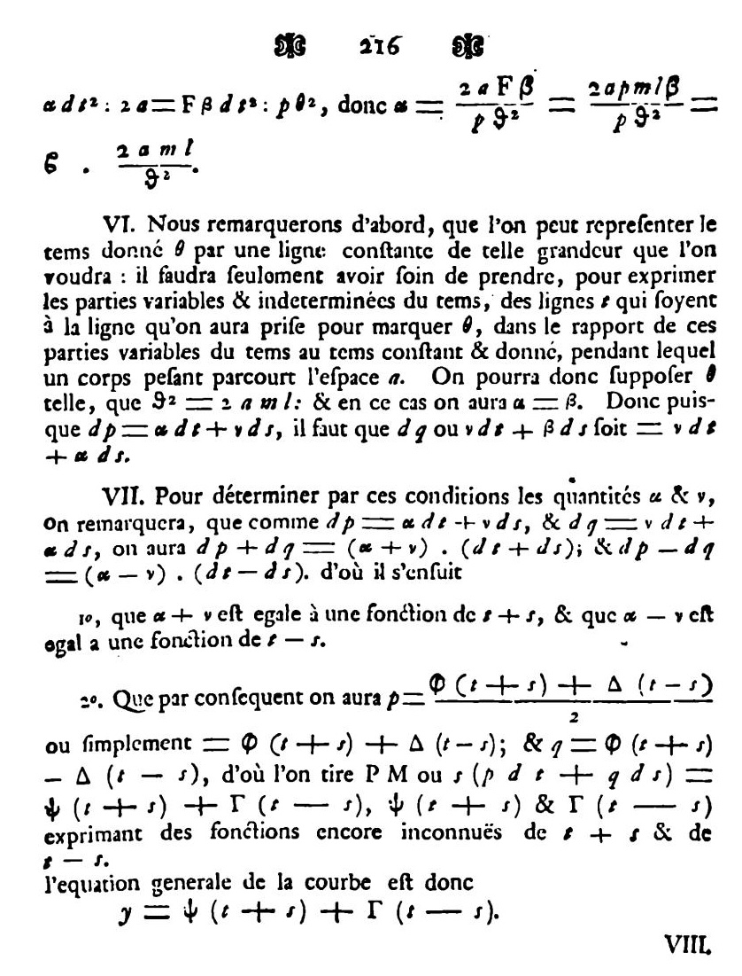
The first who solved the wave equation in an elegant way was Jean le Rond d’Alembert (1717-1783). AI (google search) had been hallucinating and telling hat d’Alembert wrote down the solution in his “wind memoire” from 1747. The correct source is an other of his papers from 1747 and you can see the formula at the bottom of the page to the right: he noticed that $f(x+t)+g(x-t)$ solves the wave equation $u_{tt} = u_{xx}$ . Now we can put this in more modern terms: d’Alembert noticed that the d‘Alembert operator $\Box = \partial_t^2-\partial_x^2$ factors as $(\partial_t-\partial_x)(\partial_t +\partial_x)$ so that the general solution of the wave equation is a linear combination of two transport equations $\partial_t u=-\partial_x u$ and $\partial_t u = \partial_x u$ . Also rephrasing in modern terms is that the Taylor theorem tells that $g(x+t) = \exp( \partial_x t) g(x)$ (Taylor just rephrasis that the one dimensional Dirac matrix $i \partial x$ is the source for translation!) So, let us introduce the self-adjoint Dirac operator $D = i \partial_x$. The transport equation $u_t = u_x$ becomes now a Dirac type equation $u_t = - i D u$ . Instead of the solution basis $\exp(i D t)$ and $\exp(-i Dt)$ we can use the real basis $\cos(Dt)$ and $\sin(Dt)$ . The explicit solution $u(t) = \cos(Dt) u(0) + D^{-1} \sin(Dt) u'(0)$ now solves the wave equation. In linear algebra courses, we usually do not write this down as such and this has also a reason, the just given solution involves the Taylor theorem and so has to assume that the initial positions and velocities are real analytic. The Fourier method allows to write down (weak) solutions for any continuous initial position and velocities. In one dimensions, d’Alembert’s direct solution is still today the most elegant approach in one dimensions and f(x+t)+g(x-t) can be matched with initial position and velocity if f,g are twice differentiable. To do so just solve f(x)+g(x)=u(0) and f'(x)-g'(x)=u'(0).

Youtube presentation from April 2023

Both the Fourier and d’Alembert method work in arbitrary dimensions and of course also in the discrete where we do not have to get into Functional analytic technicalities but focus on the basic ideas instead. The only thing we need is the square root of the Laplacian. In the continuum this is rather awkwardly done by tapping into Clifford algebras and write down Dirac matrices which from the linear algebra point of view is equivalent to tap into the exterior algebra (which is the Clifford algebra for the zero quadratic form). In the discrete, we do not have to dwell upon such acrobatics. As Dirac already felt: ugly usually just means that we are on the wrong path. The discrete world is much more beautiful. Functions on G already play the role of differential forms and the matrix D=d+d* with exterior derivative d does the job of being the square root of the Hodge Laplacian. In any case, once we have a Dirac set-up, we can write down the solution $u(t) = \cos(Dt) u(0) + D^{-1} \sin(Dt) u'(0)$ to the wave equation $u_{tt} = -D^2 u$ as before. In the calculus frame work, where D is built from exterior derivatives, we only need to worry about the Moore pseudo inverse D+ of D but that just means that we need to have u'(0) to be perpendicular to the kernel of D. The kernel of D = kernel of $D^2$ are the harmonic forms and they would lead to linear non-oscillatory solutions of the wave equation, like if the entire Newton craddle would move with constant velocity (which it does of course as we race around the sun and the sun races around the center of the galaxy) In the finite, can look also at the wave equation if the Dirac matrix D is replaced by the connection matrix L. The later is invertible and the corresponding Laplacian $L^2$ has determinant 1. Lets reiterate the remarkable fact that $\exp(-i t D) u$ is the natural “translation” of u in a finite geometry because on the real line it is the translation $u(x+t)$ as $-iD = \partial_x$ . And again: this works for any geometry with any exterior derivative, in particular also for delta sets or deformed exterior derivatives. (For connection matrices to be invertible, we need however a bit it more structure to have invertability, and simplicial complexes work just fine.)

This thanksgiving, I had been thinking a bit about this wave frame work motivated by the question whether we can use the wave equation to define sectional derivatives. The idea is to take three simplices x,y,z in G close together and look at the wave interpolation from x to y and from x to z to get two vectors v,w which define a 2-dimensional plane in the Hilbert space $l^2(G)$ which is $\mathbb{R}^n$ if $G$ has n elements. We can now start the wave equation with unit vectors from this plane and get so a 2-dimensional manifold in $\mathbb{R}^n$ . The curvature at the origin is then a notion of sectional curvature defined by the triangle x,y,z. I experimented with the simplest case where $G= \{ \{1\},\{2\},\{1,2\} \}$ is the simplicial complex $K_2$ and the Hilbert space is 3 dimensional. Now, we have 2-dimensional surfaces. In this particular case, I measured the curvatures to be positive and saw that in general, when taking other planes the curvature can also become negative. What is nice is that the curvature of two dimensional manifolds embedded into any ambient space is defined independenly of the ambient space. This is the Theorema Egregium of Gauss. Anyhow, here is the presentation from this morning:

And here is the code which gives the velocity

(* Wave interpolation,O. Knill 11/29/25 https://www.youtube.com/watch?v=Zkhvm4bzlLQ*)
CleanComplex[G_]:=Union[Sort[Map[Sort,G]]];
Generate[A_]:=If[A=={},A,CleanComplex[Delete[Union[Sort[Flatten[Map[Subsets,A],1]]],1]]];
Whitney[s_]:=Generate[FindClique[s,Infinity,All]];   Closure=Generate;    L=Length;
Connection[G_]:=Table[If[L[Intersection[G[[i]],G[[j]]]] >0,1,0],{i,L[G]},{j,L[G]}]
MatrixCos[A_]:=(MatrixExp[1.*I*A]+MatrixExp[-1.*I*A])/2;
MatrixSin[A_]:=(MatrixExp[1.*I*A]-MatrixExp[-1.*I*A])/(2I);
MatrixSinI[A_]:=Inverse[MatrixSin[A]];
Velocity[G_,i_, j_]:=Module[{x=G[[i]],y=G[[j]]},ex=Table[If[G[[k]]==x,1,0],{k,n}];
    ey=Table[If[G[[k]]==y,1,0],{k,n}]; vx=MatrixSinI[DD].(ey-MatrixCos[DD].ex); Chop[{ex,vx}]];
G=Whitney[WheelGraph[20]];n=L[G]; DD=Connection[G]; {ex,vx}=Velocity[G,1,10];
UU[t_]:=Chop[N[MatrixCos[DD*t].ex+MatrixSin[DD*t].vx]]; U=Table[UU[t], {t,0,1,0.05}];
S1=ListPlot[Transpose[U], PlotRange -> All, Joined -> True]

Youtube (“Talk to myself”) session of this morning.

Author: oliverknill