At the end of the wave front calculus paper, I added some pictures about curvature defined by wave fronts. The Bertrand-Diguet-Puiseux formula is remarkable as it shows that one can get curvature of a 2 manifold by measuring the length of wave fronts. Positive curvature means that the wave front grows slower than in the plane and negative curvature means that the wave front grows in length faster than linearly. This can be understood in many different ways, one of them being the marvelous Jacobi formula for the length of the wave front , where is the geodesic starting at in the direction and the Jacobi field satisfies the Jacobi differential equation, where is the curvature. The initial condition is J(0)=1,J'(0)=0. But the formula can also be understood by making a quadratic approximation of the surface near the point . Note that wave fronts therefore completely determine the Riemann curvature tensor in a general Riemannian manifold as if we know all the sectional curvatures, we know the Riemann curvature tensor by polarization.
The R2-D2 formula compares the length of with the length of . One looks at . This notion is more suited to be pushed to the discrete, where one can just look at in a graph, where is the graph generated by all vertices in distance 1 and is the graph generated by all vertices in distance 2. For many 2-manifolds like fullerene graphs, this gives . The same formula can also be applied for regions with boundary. This was somehow my entry point into graph geometry. The paper is here. I moved then to other things like higher dimensional Gauss-Bonnet or Poincare-Hopf formulas, then to fixed point theorems and integral geometric index expectation which also has relations to graph colorings.
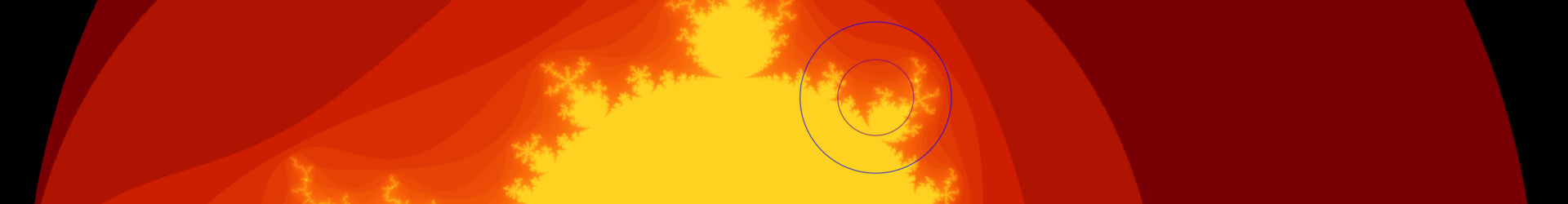
One of the things I studied mostly experimentally with the R2-D2 formula was to keep h fixed and look at the total curvature of less regular regions like polygons or fractals. The R2-D2 gives a perfectly finite curvature in even crazy cases. One could look look at the total h-curvature of the Mandelbrot set for example. An interesting question would be what the total curvature is as a function of h and whether there is a limit when h goes to zero. Classically it is of course ludicrous to talk about curvature of the Mandelbrot set or curvature of the boundary. The boundary even has 2 dimensional Hausdorff dimension by a theorem of Shishikura. Any classical notion of curvature would not apply. One could look of course at the total curvature of Green function level sets but that would just invoke the Hopf Umlaufsatz and always give the value 2pi.
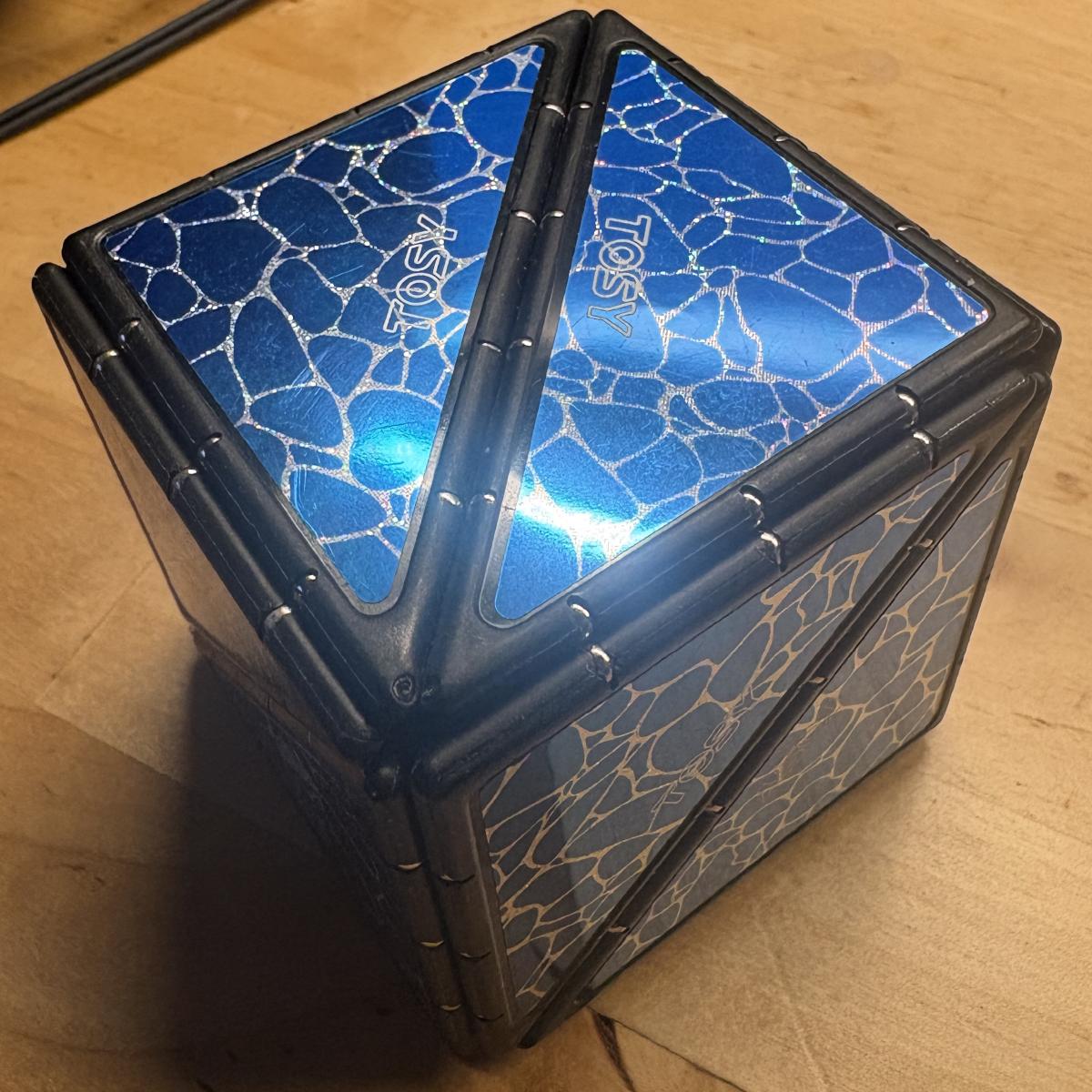
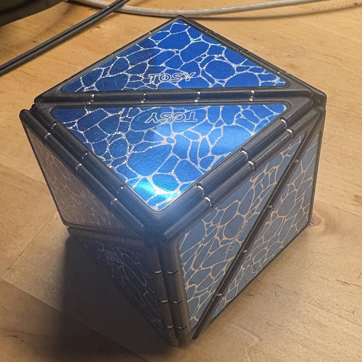
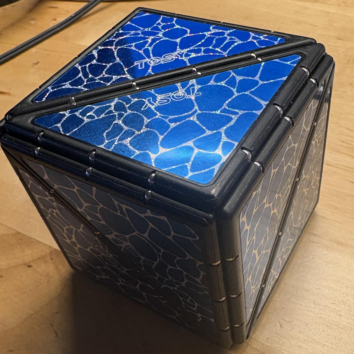
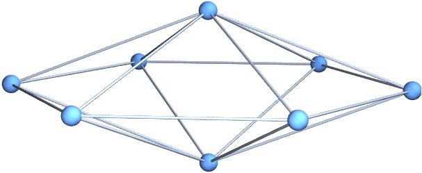
To the cube puzzle. It can generate all 64 possible triangulations by a cube. 22 of them are 2-manifolds (every unit sphere is a cyclic graph). There are two isomorphism classes. One is the prism (the join of the 1-sphere with the zero sphere. The second is the join of , where is the square (a 1-sphere) and is the disjoint union of two complete graphs. We see here already how tricky the R2-D2 curvature is. We can bend the curvature to add up to 60 if we take for the number of edges minus the number of triangles. The wave fronts can be single points, or graphs. An example of a graph which is not a 2-manifold is if three diagonals near a vertex form a triangle so that we have a subgraph. The third picture in the gallery below is an example. The usual curvature for 2-manifolds in the manifold case is in the left manifold K=1/3 (four times) and K=1/6 (four times). In the right manifold it is K=0 (two times) and K=1/3 (six times) and of course, the curvatures add up to 2 (the Euler characteristic of the sphere). This curvature has been considered by Victor Eberhard already in 2 dimensions. When I had worked on these second order curvatures, I had rediscovered it too (like probably thousands of mathematicians in the past, especially in the context of graph coloring) and then saw that the curvature works in general for arbitrary graphs! See this paper., where I had worked myself up painfully dimension by dimension up through manifold cases and then saw the general formula . A few years later I realized that the curvature had appeared already in a paper by Levitt in 1992 (but I don’t think that Levitt thought about it as a Gauss-Bonnet result). I still think having been the first to see that this is the actual Gauss-Bonnet-Chern theorem in the continuum limit if applied to even dimensional manifolds (a very special case, one does not even look at Gauss-Bonnet-Chern in odd dimensions for example or varieties etc). The link between the discrete and continuum is integral geometry. One can see the Levitt curvature as an index expectation of Poincare-Hopf indices. This picture has the advantage because it links the discrete with the continuum, we have Morse theory which introduces curvature as divisors on manifolds. If we average over all Morse functions coming from linear functions in an ambient Euclidean space in which the manifold was Nash embedded, we get to the Euler curvature (entering the Gauss-Bonnet-Chern theorem). And the same is true for networks. Take a network and embed it into an ambien Euclidean space and look at all linear functions then almost all of them (with respect to the Haar measure on all possible rotations) are functions taking different values on adjacent vertices so that Poincare-Hopf applies and the expectation of Poincare-Hopf indices is curvature. One of the latest papers mentioning such things is this on Dehn-Sommerville-Manifolds. An other mostly review is this paper on Morse and Lusternik-Schnirelmann.

| = \int_0^{2\pi} J(x(t),\theta) \; d\theta")
")
")


,\theta)")
 = - K(x(t)) J(t)")


")
 = (|2 W_t(p)| - |W_{2t}(p)|/)(2\pi r^3)")
 = |2 W_1(p)| - |W_{2}(p)|")


")


")


 = 2 |S_1| - |S_2|")


|/2+|S_2(v)|/3-|S_3(v)|/4 +....")