Spider Lemma

In order to construct the geodesic manifold of dimension k in a q-dimensional manifold, we build up the manifold in the discrete Grassmannian bundle Gr(q,k). We now do this all using the geodesic flow, which is much closer to the continuum. The simplex y in x defines (k+1)! geodesics or (k+1)!/2 geodesic arcs. In order to fit local geodesic patches together we use geodesic arcs of length 4. This produces a tree which we call “spider”. It has (k+1)! legs. The inside of the spider, the center as well as its immediate neighbors can be realized as simplices and their order will not matter any more as the legs shield them away from any attempt to be approached later by other geodesics. The set up also solves nicely the concept of parallel transport in the Grassmannian. This also is very close to the continuum. If we follow a k-dimensional plane along a geodesic, then this plane will be turned along too and as in the continuum, if we go from x to an other point z along different paths, then the parallel transport will lead to different planes. I have not implemented yet the code for generating the geodesic manifolds. It needs a bit of effort. What happens is that we build the manifold up in the Grassmannian but only use this structure during the buildup at the boundary, when extending the manifold. Physically, the geodesic manifold will return several times to the same point but with a different orientation and these instances will be far away on the geodesic manifold. This is completely analog to the continuum. Even for k=1, where we look at geodesic paths. A geodesic can hit a point again and again, coming from different directions.

Now, we understand also quite well what went wrong with the naive approach to take geodesic arcs of length 2, then close these arcs along “bones” (in the language of Regge in discrete general relativity). These closures produced too large curvature and the geodesic manifolds (they existed too!) were too small. We had constructed explicit manifolds (discretisations of higher dimensional cylinders (as boundary manifolds of geodesics in higher dimensional manifolds) for which the sectional curvature was bounded below. That was a disaster because it ment that all geodesic manifolds had an upper bound (the sectional curvatures of course satisfied Gauss-Bonnet). As pointed out several times, we want a discrete differential geometry for which the results mirror the results from the continuum. In particular, a positive lower bound for sectional curvature should produce an upper bound on the diameter of the manifold. Much further ahead, we want to study positive curvature manifolds in the discrete and see whether we can get the known positive curvature manifolds from the continuum. Basic definitions have to be simple, elegant and produce theorems. The notion of geodesic manifolds and sectional curvature are one of these absolutely crucial notions which need to be nailed down properly.

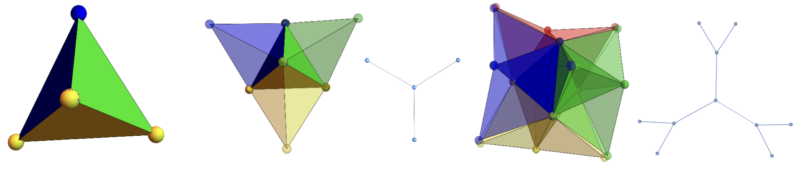
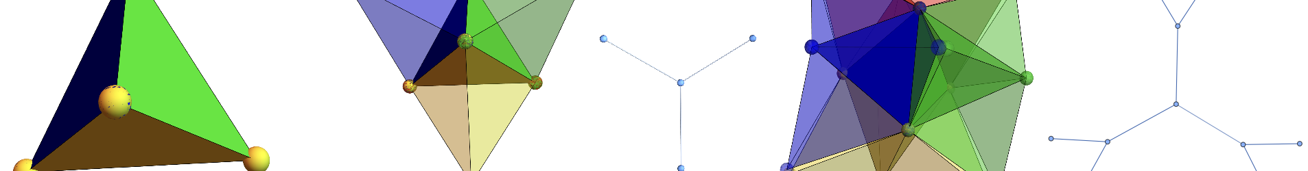
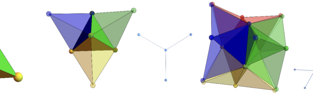
The spider lemma is explicit. For any (x,y) in Gr(q,k) this works. To build up the manifold, we start with one spider, then pick one of the legs and use this as a center of a new spider. We have now formed a larger patch. Boundary points are points in the graph for which the vertex degree is not yet k+1. The picture to the right shows how we would start in the case q=3 and k=2. Start with a simplex x=(x0,x1,x2,x3) and y=(x0,x2,x3). For every of the 3 even permutations of the triangle there is a geodesic arc through x. These three arcs of length 4 each are glued together first at x then pairwise at the legs. Now we have a spider with a center, 3 knees and 6 feet. The center and knees are now shielded away from any possible later connection as we are using geodesics. An important point of the set-up is that the geodesic flow now also produces a parallel transport of the simplex y, (the triangle here). It is always at the same location in x. It is done so that we fit with how we have defined the geodesic flow. There is a global symmetry group acting on the Grassmannian which produces different definitions of geodesic flow.