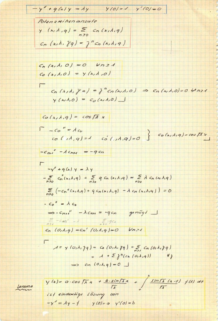
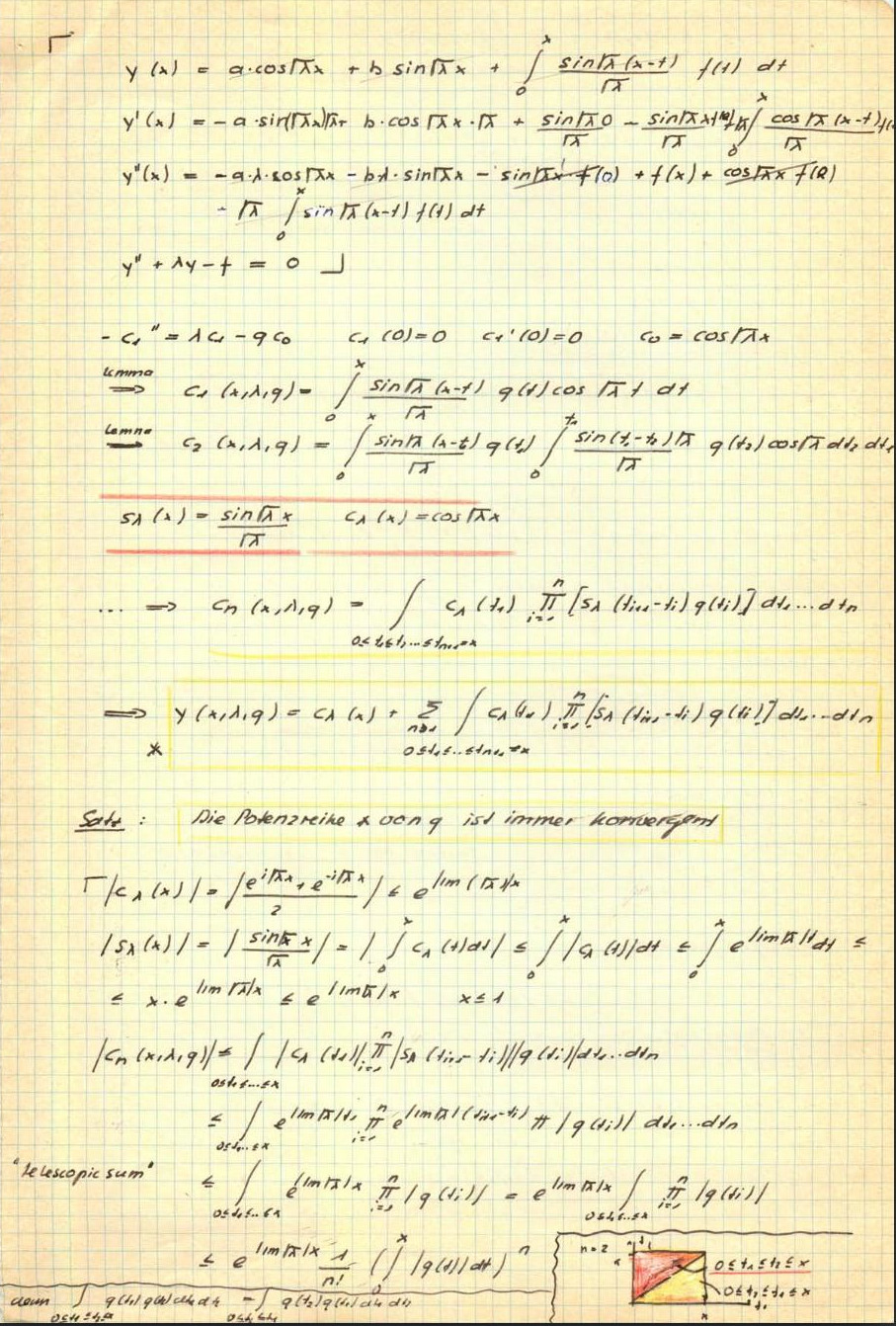
A Sturm Liouville Problem - Quantum Calculus

In our project, we looked at the deformation of exterior derivative df in a q-manifold given by $d_t f = t \phi_{q+2}(tD) df$ and saw that it satisfies the modified wave equation $u_{tt} + (q-1) u_t/t + (q-1) u/t^2 = L u$ , where $L=(d+d^*)^2=D^2$ is the Hodge Laplacian. Lets call the left hand side $A u$ . The equation $A f = g$ is a Sturm Liouville problem. Indeed, we can write $Af = g$ as $(pf')' + q f =w g$ . I was interested in solving the equation for analytic $g = \sum_{n=1}^{\infty} c_n t^{n-1}$ . Due to linearity, we only need to solve $A f = t^{n-1}$ . And this is solved by $f=-(t-t^{n+1})/(n(n+q))$ . We can so get a Taylor expansion of f.

In a previous post, I looked at $D_{tt} u = A u = 0$ , meaning zero acceleration which has the solution u(t)=a t, if a=u'(0) and of course u(0)=0 to make sense. For A u = b, which is constant acceleration, the unique solution of Au=b is $u(t) = a t + bt^2/(q+1)$ , where still a=u'(0) and 0=u(0). You see a slightly smaller acceleration. We have 1/(q+1) instead of 1/2, in the original case q=1, where $Au = u_{tt}$ . The physics intuition for the modified wave equation still works nicely. But unlike the usual wave equation for which the Kirchhoff solutions are awkward, especially in even dimensions we have a nice explicit solution $u(t,p) = d_t u(p)$ which for $(q-1)$ – forms $u$ is just the flux of $u$ through the sphere of radius $t$ . This is very intuitive: the value of the wave at time t at the position p is proportional to the flux of the initial condition u(0) through the sphere of radius t. The only thing that matters now at p is what happened at time t in distance t. This is sharp causality is and what the strong Huygens principle is about. Fortunately this is the case in three dimensions as otherwise, everything would be blurry and unsharp.

The next step of course is to exploit that $d_t$ is a bounded operator and so makes sense on the entire Hilbert space of differential forms.. For small t, like the Planck constant, the $d_t/t$ would be indistinguishable from the usual exterior derivative and so from all the physics we know. But what is nice is that for small t, the operator $d_t$ is smaller so that $D_t = d_t + d_t^*$ is small and $L_t = D_t^2$ is small. If the norm of $L_t$ is smaller than 1, then $(u,v) \to (D_t u-v,u)$ is interpolated by a related wave equation and conjugated to a unitary map. I exploited that when writing the xquantum program which is based on this paper from 1998. Unexplored is still what happens with the system $D_{tt} u = -D_t^2 u$ , where $D_t= d_t + d_t^*$ is the deformed Dirac operator and $D_{tt} = A$ is the deformed time derivative. It would be a bit of a miracle if it still would satisfy the strong Huygens principle but it would not surprise given that $D_t = \phi_{q+2}(D) D$ . We certainly also will have to look at the usual wave equation $u_{tt} = - D_t^2 u$ which has the solution $u(t) = \cos(D_t t) u(0) + {\rm sinc}(D_t t) u'(0)$ . We know that $D_t u(p)$ only involves data of u in distance $t$ from $p$ .

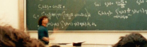
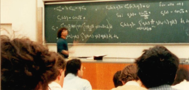
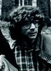
The picture to the right shows Eugene Trubowitz during an Analysis 3 lecture in 1983, where he covered Sturm-Liouville problems. I took it with my Minox camera as a student. Below are two pages from my notes from these lectures. The board in the middle third of the second page. I wrote about my undergraduate experience on this page. Our Analysis III class was Trubowitz’s first at ETHZ (he arrived in 1983) and he still learned German and walked around in the lecture hall with big mountain boots (he after all had arrived in Switzerland now …). His lectures were brilliant, original and felt like a wind of fresh air. He did what he liked and Sturm-Liouville problems were of course one of his specialities. To the right is a picture from 1984 (source). Here is an example computation showing the above statement Af=g.

q = 11; n = 23; R = -1/(n (q + n)); f[t_] := R t (1 - t^(n));
Simplify[f''[t] + (q - 1)*f'[t]/t - (q - 1)*f[t]/t^2 - t^(n - 1)]

Here is an example computation for Af=sin(t). There is an initial velocity condition which makes it bounded.

q=4; f=First[u[t] /. DSolve[{u''[t]+(q-1)*u'[t]/t-(q-1)*u[t]/t^2==Sin[t],u[0]==0,u'[0]==a}]]

In that example, a=-1/4 is the unique initial velocity which produces a bounded solution. It is seen to the right and the formula is below.

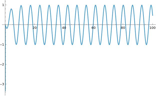
$f= -\frac{t \left(t^2-6\right) \sin (t)+3 \left(t^2-2\right) \cos(t)+6}{t^3}$ .

Author: oliverknill