


This is a bit about getting back to the story of geodesics. See “Geodesics for Discrete Manifolds” and “interacting geodesics on discrete manifolds”, all from earlier this year. I wanted to get next week on how to evolve Gaussian integer and quaternion integer particles. The quaternion primes show a nice Hadron structure while the Gaussian integers seem more aligned to the Leptons. See “quaternions and particles” from 2016, a summer when doing some experiments in number theory.
The move to cellular automaton picture is not only a philosophical one. It is much, much more effective. there are different ways to describe particles: you can make a list of particles 
The PIC method is much closer to reality than discretisations of partial differential equations. Nature after all computes with discrete particles (in the case of fluid dynamics with molecules moving around) and not with “smooth fields”. It was something Ernst Specker once pointed out during one of his classes (I don’t remember whether it had been linear algebra or one of the logic courses I took from him). He wondered, how come we take a perfectly discretized evolution system, where particles move around and use language from infinity to describe it using smooth functions and calculus, then when implementing it on a computer again discretize it and make it finite. Having used infinity as a detour, why not stay in the finite? One reason of course is that using calculus, we can use more relevant observables like moments of random variables or Fourier coefficients. Still, using the continuum is artificial, non-physical and leads to enormous mathematical difficulties. The Navier Stokes existence problem, one of the Millenium problems almost certainly does not have global solution. Why should it? It is a “man made” model after all and has little to do with the real physics if we look at the details. Fluids are not smooth fields. It is just that our inability to keep track of all these particles involves smooth statistical quantities like pressure or density. If you are a Maxwell demon, you only see particles moving around. Temperature or pressure are averages and not really fundamental.
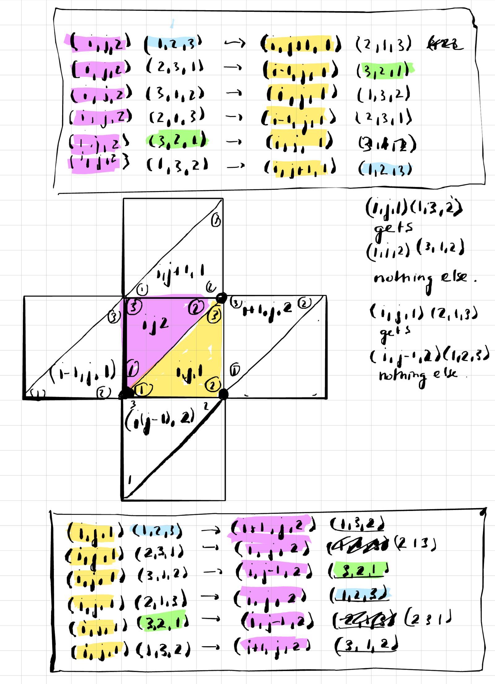
As to program the rule, the note to the right was useful (click on the picture to expand it)/ There is for each plaquette (word used in lattice gauge theory for a square) a pair of triangles A and B. Each can have 3!=6 orientations. A particle is at such a triangle and has an orientation. If it has the orientation (1,2,3) , then it moves to (2,3,4), where 4 is the anti-pode to 1. Now we have to look up how this orientation is stored in the other triangle. So, if we are on (i,j,2), the red triangle at lattice point (i,j), and have the orientation (1,2,3), then we will be in the yellow triangle (i,j+1) next with the orientation (2,1,3). In the code below we write the shift up in the second coordinate with TY and the shift down with SY. The shift right is SX and the shift down is SY. We just discussed one of the 12 cases. This is implemented as C123= TY[B213]. We of course have to use temporarily new matrices called C matrices because the A matrices will be used when writing down the new B matrices. This needs to be done when making an evolution (A,B) -> (X(A,B), Y(A,B)). One way around it is to write the evolution as a product of two involutions as I did in the general case when evolving on an arbitrary simplicial complex. I got obsessed with dihedral time when thinking about natural groups. See graphs, groups and geometry Dihedral thinking is actually quite practical from a computer science perspective as T=AB gives the inverse as BA allowing to reuse code and not having to rewrite the inverse. I did not do that in the current set-up yet, but might as the code base will become simpler, which is especially important once interactions between particles come in.
Here is the full free evolution code written on Friday. We have 12 matrices of the size M x M encoding how many particles there are in each of the 12 oriented cells at a lattice location. For a larger number of particles it is easier to keep just matrices encoding how many particles there are in each box, instead of giving the list of particles. No problem to evolve millions of particles even as this just affects how large the entries in the matrices are. I will next week talk a bit more about the interaction case. By the way Bert Hof and I once described how Cellular Automata on infinite non-periodic lattices can be evolved using finitely many data! The article was from 1995 and called Cellular automata with almost periodic initial conditions. The reason is that almost periodic data are also given by finitely many parameters. We also described the HPP model of Hardy,Pazzis and Pomeau in an almost periodic way. The HPP model by the way is very close in spirit with the geodesic evolution rule I had been looking at. Note however that in that model the number of particles at a node is finite. There are only finitely many states. Technically, the model I look at now is still a cellular automata because the total number of particles is finite. If we would look at the evolution on an infinite lattice and start with a positive density of particles then it could happen that the number of particles which can be at a node can become larger and larger. The code below however does not mind how many particles there are since we just evolve 12 integer valued matrices. The particle initial condition for example could be P := Table[If[Random[] < 0.5, Random[Integer,1000], 0], {M}, {M}]; which already gives millions of particles. The evolution does not mind and also not if we turn on interaction. If we take a million interacting particles in the continuum, we have to look at a trillion pair interactions as the number of pair interactions grows quadratically. We use “locality” to allow interactions only in each simplex itself.
[By the way, here is something about how to work on such a thing. As any programming task, this needs time to focus. Not much but having no interruption is crucial, I used 2 hours to write the handwritten document (picture above to the right) on electronic paper and an other two hours to write down the Mathematica code. But such a task needs time to focus and similarly, as when writing an exam requires time without interruption. [My differential geometry class was on Friday working on their take-home part of the exam so that I had a bit of off-time allowing to avoid being in the department]. What worked for me in this case well is to sit twice for 2 hours in a coffee shop, have ear phones on, not allow any distraction like emails, phone, people or internet. Paradoxically, this works well for me in seemingly busy places like coffee shops (I’m a Starbucks junkie and got recently shocked by removing 3 starbucks in Cambridge. In this occasion, I was working in a Starbucks in Belmont a bit of a detour when biking in from Arlington). The first batch on paper was done on Friday late morning, the second batch on the machine late in the afternoon (in clover in the science center). The code has changed since quite a bit as I also implemented already the interaction part. But this makes the program look more complicated, about twice as long. It is important for later to keep the first version. In a few months, I might have forgotten how this cellular automata code was written. ]
M = 100; Q = Table[0, {M}, {M}];  P :=  Table[If[Random[] < 0.002, 1, 0], {M}, {M}];
A123 = P; A132 = P; A213 = P; A231 = P; A312 = P; A321 = P;
B123 = P; B132 = P; B213 = P; B231 = P; B312 = P; B321 = P;
TX[A_] := Transpose[RotateLeft[Transpose[A]]];     TY[A_] := RotateLeft[A];
SX[A_] := Transpose[RotateRight[Transpose[A]]];  SY[A_] := RotateRight[A];
DoEvolution := Module[{ },
   C123 = TY[B213]; C231 = SX[B321]; C312 = B132;
   C213 = SX[B231]; C321 = B312; C132 = TY[B123];
   B123 = TX[A132]; B231 = A213; B312 = SY[A321];
   B213 = A123; B321 = SY[A231]; B132 = TX[A312];
   A123 = C123; A132 = C132; A213 = C213; A231 = C231; A312 = C312; A321 = C321;
   AAAA =A123+A132+A213+A231+A312+A321+B123+B132+B213+B231+B312+B321];
DoEvolution;U = Table[DoEvolution;     MatrixPlot[AAAA], {500}];
Animate[Show[U[[k]]], {k, 1, Length[U], 1}]