Connection and Hodge Laplacians

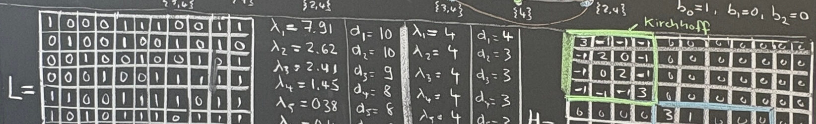
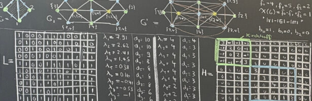
Before we start, here is the code which generated the two matrices on the board of the talk. 5 lines for the Hodge Laplacian, 1 line for the Connection Laplacian. This works for any simplicial complex.

Generate[A_]:=If[A=={},A,Delete[Union[Sort[Flatten[Map[Subsets,A],1]]],1]];
Whitney[s_]:=Generate[FindClique[s,Infinity,All]];       L=Length;      T=Transpose;
Connection[G_]:=Table[If[L[Intersection[G[[i]],G[[j]]]]>0,1,0],{i,L[G]},{j,L[G]}];
F[G_]:=Delete[BinCounts[Map[L,G]],1];      S[x_]:=Signature[x];      Q[A_]:=A.A;
s[x_,y_]:=If[SubsetQ[x,y]&&(L[x]==L[y]+1),S[Prepend[y,Complement[x,y][[1]]]]*S[x],0];
Hodge[G_]:=Module[{f=F[G],d,n=L[G]},d=Table[s[G[[i]],G[[j]]],{i,n},{j,n}]; Q[d+T[d]]];
K=CompleteGraph[{1,2,1}];G=Whitney[K];A=Connection[G];B=Hodge[G];Map[MatrixForm,{A,B}]

Not only in physics, also in mathematics, there is a fundamental distinction between Fermionic and Bosonic objects. The calculus of Archimedes dealing with area and volumes is of Bosonic nature. It does not matter whether you add up the slices of a solid left to right or right to left. The dx was sign-less and $\int_a^b A(x) dx$ is an integral geometric quantity. The calculus of Newton and Leibniz however was Fermionic. It led to the fundamental theorem of calculus, where dx is a 1-form and where $\int_a^b f(x)dx$ comes with a sign as $\int_a^b f'(x) dx=f(b)-f(a)$ illustrates. The two flavors of summing up are in calculus courses mixed up. In multi-variable calculus, the arc length or surface area or volume are integral geometric Bosonic quantities, while line integrals and flux integrals are of differential geometric Fermionic nature meaning that orientation is relevant. In calculus we hide this and some legacy textbooks like Stewart puzzle us by putting scalar surface integrals like $\iint_S f(\vec{r}(u,v)) dS$ close to flux integrals $\iint_S \vec{F}(\vec{r}(u,v)) \cdot \vec{dS}$ . The former integral is a generalization of the surface area and for example sums up the charge density over a surface. The later depends on orientation like the flux of a fluid through a surface. You can try this out ask for the surface area of the cone $x^2+y^2=z^2, |z|<1$ and see computations like this $\vec{r}(u,v) = [v \cos(u),v \sin(u),v]$ , $\vec{dS}= [v \cos(u),v \sin(u),-v], dS=\sqrt{2} v$ , $\iint_R dS = 2\pi \sqrt{2} \int_{-1}^1 v \; dv = 0$ which of course is nonsense as the surface area is positive. I wrote about this 9 years ago already here (on this blog) and in this youtube video from 2 years ago. This is actually a very important thing to consider in course design. Our first calculus course Math 1a (I taught this a couple of times like here) is a course which is actually quite a Fermionic course as it aims at the fundamental theorem of calculus. Our second calculus course Math 1b (I taught this only twice but did not design the course) is a “Bosonic course”. It uses integration mostly to compute densities. It also deals with series in a Bosonic meaning in that the order in which the sum is added up does not matter. One difficulty to go then to multivariable 21a is that the later is both using Bosonic and Fermionic calculus. The integral theorems actually integrate differential forms, the surface area and arc length integrals as well as volume integrals are still integral geometric and orientation oblivious.

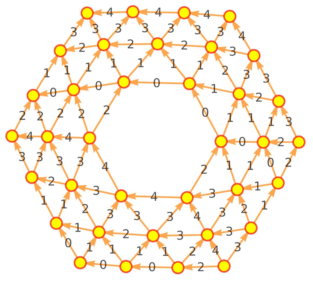
Now it is only in the discrete, on a quantum level so to speak that the distinction between Bosonic and Fermionic approaches becomes crystal clear. If we compute the length of a path in a network, we do not care about orientation. We just count the number of edges which are in the path. To compute the surface area of a surface, we just count the number of triangles. More generally, the f-vector, encoding the number of k-dimensional parts of space is just counting. The orientation of these constituents of space are irrelevant for this. Also if we would weight the individual simplices with numbers and add up these “densities” we would still get something that is orientation irrelevant. It is “Bosonic”. This completely changes if we look at the integral theorems in the discrete. Lets look at the problem I gave to my summer school class as an optional problem in the final exam [PDF] (there was a 15 minute exposure to discrete calculus at the end of some review). The problem had been to compute the flux of the curl of the vector field over the surface in the picture. A vector field is a number attached to an oriented edge. The line integral along a curve sums up these values. The curl of a vector field is a function on triangles obtained as the line integral along the boundary. In the example, the sum of the curls can be computed by adding up two line integrals along the boundary. The outside counterclockwise, the inside clockwise. The result was 24. Bosonic quantities in this example are the surface area (48) and boundary length (that this is 24 is an accident. I had chosen the vector field values randomly.

Now to the video recorded last Saturday: I use the Hodge Laplacian since the very beginning of my work on discrete calculus (now almost 15 years). The connection Laplacian came in in the winter 2015/2016. I noticed the unimodularity which needed a few months during 2016 to be proven. I must add that the summer of 2016 had been disrupted a bit after reading the book of Mazur and Stein on the Riemann hypothesis. My review is here. One of the problems in that book was to come up with your own problems about prime numbers. I performed during the early summer a few experiments in number theory. The most interesting problem I came up with (for me) were Goldbach statements for Gaussian Hurwit, Octavian and Eisenstein primes which are all new. I actually tried to send this to a journal once whereas the referee essentially said that there is too much information. It reminded me about the famous “too many notes” scene in “Amadeus” …

The topic of the talk was about the Hodge Laplacian $H=D^2$ and the Connection Laplacian $L$ of a finite abstract simplicial complex. There are some remarks about comparing the two. One of the reasons to see the connection Laplacian as something Bosonic is that if you look in one dimensions at $L-L^{-1}$ , you get the signless Hodge Laplacian, which is an orientation oblivious and so Bosonic notion. I would have really loved to see a direct relation between the connection Laplacian and some sort of signless Hodge Laplacian in higher dimensions but that has not surfaced yet. The invesigation of the spectrum of these Laplacians will certainly come back for me.

Author: oliverknill