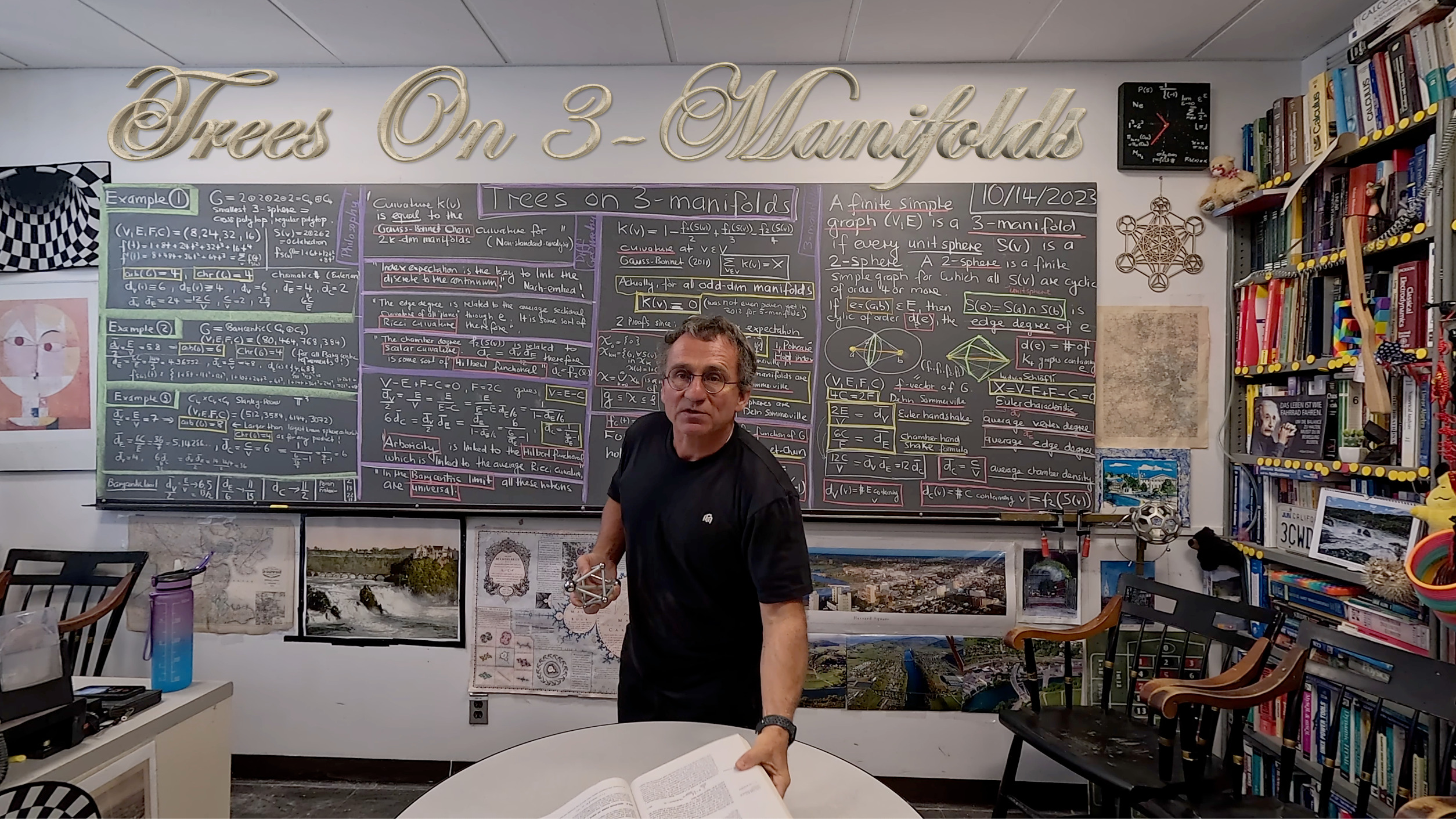
Trees on 3-manifolds - Quantum Calculus

We started to look at the problem to find the arboricity of 3-manifolds. First of all, we are interested in the functional E/V, where E is the number of edges and V is the number of vertices. The topology and differential geometry of 3 manifolds is much more rich than the topology of 2-manifolds, where we knew the arboricity was 3 or 4. In the case of 3-manifolds, already for 3-spheres, the arboricity can be 4,5,6, or 7 but we do not know whether it can be 8. For 2-tori there are examples of arboricity 7 (through Barycentric refinements) and arboricity 8 (an explicit example).

The combinatorics of 3-manifolds is encoded by the f-vector (V,E,F,C), where V is the number of vertices ( $K_1$ subgraphs), E is the set of edges ( $K_2$ subgraphs) , F is the set of triangles ( $K_3$ subgraphs) and C is the set of tetrahedra ( $K_4$ subgraphs). The Euler characteristic was already defined in higher dimensions by Ludwig Schlaefli. For 3-manifolds, graphs for which all unit spheres are 2-spheres, the Euler characteristic is $X = V-E+F-C$ . For 3-manifolds, the Euler characteristic is always zero. There are many ways to see this, using cohomology, using Poincare-Hopf (the index $j_f = i_f+i_{-f}$ is always zero for manifolds). Since Gauss-Bonnet curvature $K(v)$ integrating up to Euler characteristic $X(G) = \sum_{v \in V} K(v)$ is the expectation $K(v) = {\rm E}[i_f(v)]$ of Poincare-Hopf indices had been my first explanation that curvature is constant zero for odd-dimensional manifolds. There is a index formula which is for odd d-dimensional manifolds the Euler characteristic of a manifold of dimension d-2. There is also a Dehn-Sommerville explanation. See the sphere formula for a newer explanation.

In the movie, I throw in some low hanging fruits like a formula for the edge degree of an edge $e=(a,b)$ . It is the length of the circle $S(a) \cap S(b)$ . By definition of manifolds, the intersection of two adjacent spheres S(a) and S(b) in the manifold is a unit sphere in each of the spheres and so a sphere of co-dimension 2. In the case of 3-manifolds, this is a one dimensional sphere, meaning a circular graph with 4 or more vertices. Interesting is the case of 4-manifolds (maybe I say more about this next week, where the center manifold is a 2-dimensional surface at every point). Analog to the Euler handshake formula $2E/V = \overline{d_V}$ showing that the half of the vertex degree average is E/V, we have a higher dimensional version $6C/V = \overline{d_E}$ gives the average edge degree. I’m fascinated by quantities like E/V or C/V because they are universal in the Barycentric limit. One can express the limiting quantities in terms of $A=\left[ \begin{matrix}1 & 1 & 1 & 1 \\0 & 2 & 6 & 14 \\0 & 0 & 6 & 36 \\0 & 0 & 0 & 24 \\ \end{matrix}\right]$ which has the Perron-Frobenius eigenvector $[ 2,13,22,11 ]$ giving the limiting quantities E/V=13/2 and C/V=11/2. For any 3-manifold or more generally, for any graph of maximal dimension 3, in the Barycentric limit, the arboricity is 7. We see that for a small 3-dimensional torus with f-vector $(512, 3584, 6144, 3072)$ , we have E/V=3584/512=7 meaning that the arboricity must be 8. Already after one Barycentric refinement with f-vector $(13312, 87040, 147456, 73728)$ which gives an $E/V=87040/13312=85/13=6.53846$ which indicates arboricity 7 (we do not know of course for sure yet because it could be that some subset of vertices generates a graph with larger arboricity but I have never seen an example of a manifold, where the arboricity is not decided by the ration E/V already which is a strong local maximum for manifolds and a good candidate for a global maximum.

Speaking of manifolds: Having grown up as a mathematical physicist (we had as mathematicians in the ETH focus on one of the three choices Computer Science, Statistics or Mathematical physics to which I chose the later), physical motivation is always important for me. I mention during the presentation Regge calculus, even so I must admit not be a fan of any type of discrete mathematics which uses the continuum as a crutch. For me, talking about “angles” or “lengths” using Euclidean intuition is nothing else than a numerical scheme. And numerical schemes are almost always incredibly ugly. Look at a typical numerical analysis book and you know what I mean. When looking at numerical schemes for ordinary or partial diferential equations, it often comes with nasty notation and explaining why the continuum calculus is so much more attractive. This comes already to light in single variable calculus, where one worries about quantities like $\Delta x = (b-a)/n$ in numerical schemes and where the elegant integral $\int_a^b f(x) \; dx$ becomes the ugly sum $\sum_{k=1}^n f(x_k) \Delta x$ which is filled with additional definitions like $x_k = a + k \Delta x$ and $\Delta x = (b-a)/n$ . In higher dimensions especially, and when trying to make the numerical schemes more efficient and numerically stable, one gets into hell (from the point of view of the mathematician of course and not for the engineer, beauty is not always the same than effectiveness).

Sometimes however one has to disagree with the cliche that beauty is the anti-pode to effectiveness. An example is Gauss-Bonnet, especially in higher dimensions, where we have to deal with a theorem that carries quite a bit of baggage. I speak here as somebody who has really implemented and worked with explicit computer implementations for differential geometry and struggled to get effective code to compute the Gauss-Bonnet-Chern integrand (not that difficult) but then to integrate this over a concrete manifold (quite hard, even in very simple cases like general ellipsoids). Here and here are some writings about this. In the discrete the Gauss-Bonnet story can be incredibly elegant. Instead of talking about the Euler characteristic X, we better talk about the generating function of the f-vector which is the f-function $f(t) = 1+f_0 t + f_1 t^2 + f_2 t^3 + f_3 t^4$ which in the case of 3-manifolds, it is $f(t) = 1+V t + E t^2 + F t^3 + C t^4$ (isn’t it great to have single variable calculus matter so much in combinatorics? Look at this document for a math 1a course [PDF]).

The theorem I wanted to pitch a bit also during the presentation is that the f-function of an arbitrary graph satisfies the Gauss-Bonnet property

$f_G'(t) = \sum_{v \in V} f_{S(v)}(t)$ .

This is by far not yet the most general form. I had generalized this to multi-dimensional valuations, where the generating functions are functions of several variables and where the Euler characteristic is replaced by higher charactieristics or to cases, where the energy $w(x) = (-1)^{dim(x)}$ is replaced by some function $h(x)$ . This energy which enters the Euler characteristic $X(G) = \sum_{x \in \mathcal{G}} w(x)$ of the graph ,sums over the finite abstract simplicial complex $\mathcal{G}$ consisting of all vertex sets of complete sub-graphs of the graph (which by the way for me as a non-graph theorist by birth was always the most natural thing to do. Who the heck would think about a graph as a one dimensional object. Well, graph theorists often do and are proud about it. Not to mention that my papers (when I had still tried to submit papers to journals) did not even warrant a referee report.

Here is mathematica code which allows an interested reader to experiment. I have published this maybe already a half a dozen times, also embedded in my ArXiv papers. Here are a dozen lines which allow to compute curvatures, f-vectors, Euler characteristic etc. The 12 lines were written so that it is from the code itself clear what is done. You should be able to see what each procedure does without further explanation. It should run with any recent Mathematica version (currently 13.3.0) and is written in a way that it will run with any future mathematica version. The code also reminds about the Dehn-Sommerville invariants which are obtained as the eigenvectors of the Barycentric refinement operator.

UnitSphere[s_,v_]:=Module[{U=NeighborhoodGraph[s,v]},If[Length[VertexList[U]]<2,Graph[{}],VertexDelete[U,v]]];
UnitSpheres[s_]:=Module[{V=VertexList[s]},Table[UnitSphere[s,V[[k]]],{k,Length[V]}]];
Generate[A_]:=Delete[Union[Sort[Flatten[Map[Subsets,A],1]]],1]; 
WhitneyComplex[s_]:=Generate[FindClique[s,Infinity,All]];
Fvector[s_]:=Delete[BinCounts[Map[Length,WhitneyComplex[s]]],1];
Ffunction[s_,x_]:=Module[{f=Fvector[s]},If[Length[VertexList[s]]==0,1,1+Sum[f[[k]]*x^k,{k,Length[f]}]]];
Curvature[s_,x_] :=Module[{g=Ffunction[s,y]},Integrate[g,{y,0,x}]];
Curvatures[s_,x_]:=Module[{S=UnitSpheres[s]},Table[Curvature[S[[k]],x],{k,Length[S]}]];
EulerChi[s_]:=Module[{f=Fvector[s]}, -Sum[f[[k]](-1)^k,{k,Length[f]}]];
DehnSommervilleQ[s_]:=Module[{f},Clear[x];f=Ffunction[s,x];Simplify[f]===Simplify[(f /. x->-1-x)]];
BarycentricOperator[n_]:=Table[StirlingS2[j,i]*i!,{i,n+1},{j,n+1}];
DehnSommervilleInvariants[n_]:=Eigenvectors[Transpose[BarycentricOperator[n]]];

And here are some example computations. First a random graph, showing off Gauss-Bonnet for the F-function, then showing the Dehn Sommerville invariants for 4 manifolds, then a three sphere

s=RandomGraph[{10,20}]; {Ffunction[s,x],1+Total[Curvatures[s,x]]}
{EulerChi[s],-Total[Curvatures[s,x]] /. x->-1}

MatrixForm[Transpose[Reverse[DehnSommervilleInvariants[4]]]]

threesphere=UndirectedGraph[Graph[{1->3,1->4,1->5,1->6,1->7,
1->8,3->2,3->5,3->6,3->7,3->8,4->2,4->5,4->6,4->7,4->8,5->2,
5->7,5->8,6->2,6->7,6->8,7->2,8->2}]]; 
{EulerChi[threesphere],DehnSommervilleQ[threesphere],Ffunction[threesphere,t]}

Author: oliverknill