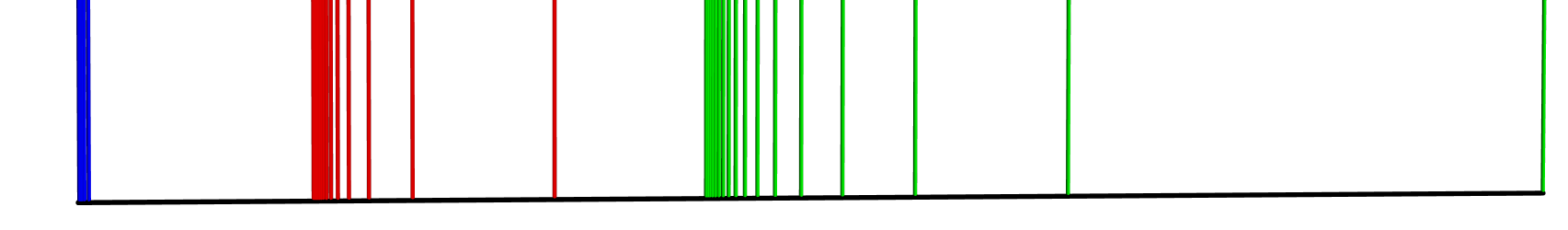
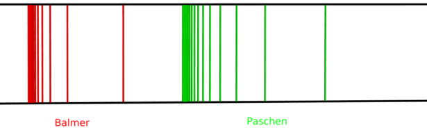
3D Dirac operator - Quantum Calculus

The three dimensional space $\mathbb{R}^3$ is important because we live in it. With the scalar Laplacian $-\Delta$ in dimension q=3, the Hydrogen operator $-\Delta + 1/r$ (leaving out constants) essentially explains the periodic system of elements and so the starting point of chemistry. The eigenvalue difference $1/n^2 - 1/m^2$ explain spectral lines (like Lyman (UV light) , Balmer (visible light) , Paschen (infrared light) ). The integral operator expressions for the inverse of the Laplacian explain why the electromagnetic or gravitational potentials have the form $1/r$ . The three dimensional integral calculus is taught in multi-variable calculus courses, where the exterior derivative grad, curl and div appear. One usually does not write down the Dirac operator on all differential forms. There are 0 forms, 1 forms, 2 forms and 3 forms. We usually identify 0 and 3 forms and 1 and 2 forms. The curl of a vector field is still considered to be a vector field. The Dirac operator in flat 3 dimensional space is $D = \left[ \begin{array}{cccc} 0 & -{\rm grad}^* & 0 & 0 \\ {\rm grad} & 0 & {\rm -curl}^* & 0 \\ 0 & {\rm curl} & 0 & {\rm -div}^* \\ 0 & 0 & {\rm div} & 0 \end{array} \right]$ . The Hodge Laplacian $L=D^2$ has 4 diagonal blocks containing the scalar Laplacian $L_0 = -\Delta$ . For 3-forms, it looks the same just $L_3 f dxdydz = -\Delta f dxdydz$ . On 1-forms and 2-forms which in multi-variable calculus always are identified as “vector fields”, one would write there $L_1 ( P dx + Q dy + R dz) = -\Delta P dx -\Delta Q dy - \Delta R dz$ and similarly for 2-forms $P dydz + Q dxdz + R dxdy$ . The solution of the wave equation in 3 dimensional space $u_{tt} = \Delta u$ can be written down conveniently as $u(t) = \cos(Dt) u(0) + t {\rm sinc}(Dt) u'(0)$ . And now we can note that $\cos = \phi_1$ and ${\rm sinc}= \phi_3$ are Bessel functions. This triggered me to talk on Saturday about a PDE riddle. The path $u(t) = \phi_k u(0)$ is a solution of a modified wave equation $u_{tt} = - D^2 u - (k-1) u_t/t$ as the computation in the box below shows. I had hoped that $u(t) = \phi_k u(0) + t \phi_{k+2} u'(0)$ would more generally solve this wave equation; but this did not pan out: for the velocity part, it only fits for $k=1$ , where it is the usual wave equation and where $\phi_{3} ={\rm sinc}$ is the sinc function.

A PDE attempt:

Motivated by the fact that $u(t) \phi_1(tD) u(0) + t \phi_3(tD) u''(0)$ solves the wave equation $u_{tt} + D^2 u=0$ on an arbitrary Riemannian q-manifold, we attempted to see whether in general, $u(t) = \phi_k(tD) u(0) + \phi_{k+2}(tD) u'(0)$ satisfies a modified PDE. Here, $\phi_q(r)$ solves the Bessel differential equation $\phi''(r) + (q-1) phi'(r) /r + phi(r) =0$ with the initial condition $\phi(0)=1, \phi'(0)=0$ . The first cases are $\phi_1(r) = \cos(r)$ , $\phi_2(r) = J_0(r)$ , $\phi_3(r) = {\rm sinc}(r) = \sin(r)/r$ , $\phi_4(r) = 2 J_1(r)/r$ and $\phi_5(r) = \frac{\sin (r)-r \cos (r)}{r^3}$ . Since the d’Alembert type formula $u(t) = \phi_1(tD) u(0) + t \phi_3(tD) u'(0)$ satisfies the wave equation $u_{tt} = - D^2 u$ on a general Riemannian manifold $(M,g)$ with Dirac operator $D=d+d^*$ , the square root of the Hodge Laplacian $d d^* + d^* d$ , it was tempting to explore whether $\phi_k(tD) + \phi_{k+2}(tD)$ satisfies this PDE. On Saturday morning, I thought it does, but if done correctly, there is an annoying single term $\phi_{q+2} u'(0) (q-1)/t$ left, when trying with the wave type equation $u_{tt} + D^2 u + u_t (q-1)/t = 0$ . (The computation is below). The reason, why I would have liked it is because it would give more intuition about why $D_t f = \phi_{q+2}(tD) Df$ is a good deformation of the Dirac operator. What we know is that $D_t f(p)$ is completely determined by $f$ only on $W_t(p)$ the wave front. In dimension $q$ , we need $\latex \phi_{q+2}$ when doing sphere averages and I still wonder why $q+2$ and not $q$ in dimension $q$ . It is clear in 1-dimension, where $\phi_3= {\rm sinc}$ is needed to get the discrete derivative $[f(x+t)-f(x-t)] /2$ .

Upshot: the form $u(t) = \phi_q(tD) f$ satisfies the PDE $u_{tt}+D^2 u + (q-1) u_t/t=0$ with $u(0)=f$ . The path $u(t)=t \phi_{q+2}(tD) f$ does not satisfy this PDE with initial velocity $u_t(0)=f$ however. The question had been triggered by the fact that the expression $d_t f = \phi_{q+2} (tD) df$ is a nice deformed exterior derivative that uses the wave front at distance t.

Update of February 24, 2025: I was happy of having had 3 hours uninterrupted focused work in a coffee shop at Harvard square on February 24th and could try again. The fact that the computation below was so close to work had indicated strongly that there is a PDE that should work. My “hunch” turned out to be ok and and it indeed does. What I do in such a case is do “wishful thinking” and just try, then try again, compute various expressions and try to modify them to add to zero. It is indeed a “puzzle” like any other. It is just here that the parts of the puzzle are mathematical expressions. The modified wave equation that works is $u_{tt} + D^2 u + (q-1)(u_t/t-u/t^2)=0$ . If u(0)=0 and $u_t(0)$ = D f for an arbitrary differential form f, then the solution $u_t(t,x) = D_x f = \phi_{q+2}(tD) tD f, u_t(0,x)=Df, u(0,x)=0$ is the deformation of the Dirac operator we have looked at this winter (starting in December 2025). Now, we can turn things around and have a PDE on arbitrary q-manifolds that satisfy the strong Huygens principle in all dimensions: the value of $u_t(t,x)$ depends only on the value of $u_t(0,y)$ with $y \in W_t(x)$ , the wave front. It also follows that the solution of that wave equation has an explicit bounded operator as the wave operator. And this operator explains somehow the weird fact that the Bessel function $\phi_{q+2}$ matters on q-manifolds. (It already did for the usual wave equation $u_{tt} + D^2 u=0$ , where the explicit solution is $u(t,x) = \phi_1(tD) u(0) + t \phi_3(tD) u'(0)$ . ) I do not repeat any hand computation as it is a bit more messy than the box below from last Sunday. But here is a 3 line Mathematica verification. It can hardly be simpler but still strange how the usual wave equation is modified using u and $u_t$ parts. First we define the Bessel function $phi_{q+2}(tD)$ , then set $u = t \phi_{q+2}(tD) Df$ (in mathematica, I use d for the Dirac operator, as D is reserved for derivative). Then we show that u(0)=0 and $u_t(0) = Df$ encodes the usual traditional standard exterior derivative in the Riemannian manifold. Then we check that the modified exterior derivative this satisfies the modified wave equation. If you want to look up expressions like D[u,{t,2}] encoding $u_{tt}$ they are for q=10 already quite complicated:

q=10; g=First[f[r]/.DSolve[{f''[r]+(q+1)f'[r]/r+f[r]==0,f[0]==1,f'[0]==0},f[r],r]];
phi=g/.r->d t;  u=t phi d f;    {Limit[u, t -> 0],   Limit[D[u,t],t->0]}
FullSimplify[D[u,{t,2}]+d^2*u+(q-1)D[u,t]/t-(q-1)u/t^2==0]

End of update from February 24th. The rest was written Sunday:

Just to recall, the starting point had been that $d_t f = \phi_{q+2} (tD) df$ is the flux of $f$ through $W_t(p)$ if $f$ is a $(q-1)$-form. This was a consequence of the Jeffrey Ovall formulas for sphere or ball averages. One can deduce from this that the Huygens property holds for all differential forms and not only q-1 forms. Using the magical Cartan formula for the Lie derivative $L_X = i_X d + d i_X$ , one can in generalsee by taking inner derivatives that also for general k-forms, the formula $d_t f$ produces an exterior derivative that only uses $f$ on the wave front: one just has to write every differential form as a linear combination of decomposable forms i_X g, where g is invariant under the flow of X like $i_{e^1} g(y) dx= g(y)$ or $i_{e^2} g(x) dy = g(x)$ or $i_{e^1+e^2} g(x-y) (d(x+y)) = g(x-y)$ in the case $q=2$ and derive the Huygens principle for $k=0$ forms if it is known for $k=1$ forms. Why do we see the Bessel case $q+2$ in the sphere averages in dimension $q$ ? The PDE $u_{tt} + D^2 u + u_t (q-1)/t$ almost works for the velocity. It does for position, but for velocity there is a term left. If the initial velocity $u_t(0)=0$ is zero, then $u(t) = \phi_q(tD) u(0)$ satisfies this modified wave PDE. It would have been nice (and was wishful thinking triggered by the 1- dimensional case) to explain better the q+2 Bessel solution appearing in the exterior derivative $d_t f = \phi_{q+2}(tD) df$ that is the center of attention as it has the property that $d_t f(p)$ only depends on the wave front $W_t(p)$ . There is a cancellation explaining a bit the shift from the q-Bessel equation $f''+(q-1) f/r + f=0$ to the (q+2)-Bessel equation $f''+(q+1) f/r = f=0$ solved by $\phi_{q+2}$ , but it is not enough.

Attempt: is it true that u = f_q u(0)  + t f_{q+2} u'(0)  = f X + t g Y
solves the PDE           u_tt + D^2 u + u_t (q-1)/t=0   where f_q  solves
the Bessel equation f''(r) + (q-1) f'(r)/r  + f(r) = 0,  f(0)=1, f'(0)=0         ?

Write u(0) = X and  u'(0) = Y   for the initial position and initial velocity.
Write simply f = f(tD) =f_q(tD)  and     g = g(tD) = f_{q+2}(tD) and use

Bessel  f''(tD) + (q-1) f'(tD)/(tD) + f(tD) = 0                (*)
Bessel  g''(tD) + (q+1) g'(tD)/(tD) + g(tD) = 0                (**)
chain rule :   d/dt f(tD) = f'(tD) D  and   d^2/dt^2  f(tD) =    f''(tD) D^2  

       POSITION                          MOMENTUM
------------------------------------------------------------------------------
u    = f       X                   + t g     Y    
u_t  = f'  D   X                   + t g'  D Y               +   g    Y     
u_tt = f'' D^2 X                   + t g'' D^2 Y  +  g' D Y  +   g' D Y
------------------------------------------------------------------------------            

Multiply the first equation by D^2, the second by (q-1)/t and switch q-1 to q+1
with      t g' D^2 Y (q-1)/(tD)  =   t g' D^2 Y (q+1)/(tD)    - 2 g' D Y    

------------------------------------------------------------------------------            
D^2 u       = f   D^2 X            + t g   D^2 Y    
u_t (q-1)/t = f'  D^2 X (q-1)/(tD) + t g'  D^2 Y (q+1)/(tD) + g Y (q-1)/t  -   2g' D Y
u_tt        = f'' D^2 X            + t g'' D^2 Y            + 2g' D Y  
------------------------------------------------------------------------------

              Bessel  (q-1)          Bessel (q+1)   
 Adds to 0    Add to 0               Add to zero           g Y (q-1)/t
 by PDE       by (*)                 by (**)                  Remains

A PDE attempt:

Author: oliverknill