Discrete Calculus
I had been busy teaching the new course math 22a last fall. Related to quantum calculus are the units Unit 33: discrete I and Unit 37 Discrete II where multi-variable calculus isdone on graphs. There was also a short presentation adapted from the final review:
Cartan’s magic formula
Related to quantum calculus is the topic of Cartan’s magic formula which has a surprisingly simple implementation in the discrete. This formula gives an expression of the Lie dervative LX in terms of the exterior derivative d and an inner derivative iX. The Magic formula of Cartan shows that the Lie derivative is a type of Laplacian and a square of a Dirac type operator d+iX. This is kind of neat as if one has a Dirac operator, then one can write down immediately formulas for the corresponding wave equation. It essentially is a Taylor expansion. Teaching the topic of the multi-variable Taylor expansion actually led to this note. By the way, everything is also illustrated with actual Mathematica code. Just download the LaTeX source of the paper to get the code. It is simple text as I don’t trust mathematica notebooks. Their format will change over time. [The technical specifications of .nb files changed during the last decades I used Mathematica. One can hardly open a 20 year old 1.2 notebook any more, but there is no problem with 20 year old plain code as this is just language independent of technical implementation.]
Elie Cartan (1869 – 1951) is the father of differential forms. The idea was published in his “Les systemes differentiels exterieurs et leur applications geometriques“.
Given a compact Riemannian manifold or a graph, we have both an exterior derivative $d$ as well as an interior derivative $i_X$ for every vector field X. The map $d$ maps $\Lambda^p$ to $\Lambda^{p+1}$ and the map $i_X$ like $d^*$ maps $\Lambda^{p+1}$ to $\Lambda^p$. All these derivatives satisfy $d^2=(d^*)^2=i_X^2=0$. We can now form two type of Dirac operators and Laplacians
$$ D_X = d + i_X , L_X = D_X^2 = d i_X + i_X d $$
$$ D = d + d^* , L = D^2 = d d^* + d^* d $$
The equation $L_X = d i_X + i_X d$ is called the Cartan’s magical formula. In the special case $p=0$, where $L_X$ and $L$ are operators on scalar functions, we have $L_X f(x) = d/dt f(x(t))$, where $x'(t) = X x(t)$ is the flow line of the vector field $X$.
Applying $i_X$ is also called a contraction. For scalar functions, $f \to D_X f = i_X df = df(X)$ is a directional derivative. It follows from the Cartan formula that the Lie derivative commutes with $d$ because $L_X d = d i_X d = d L_X$. We can also check that Lie derivative satisfies $L_[X,Y] = L_X L_Y – L_Y L_X$ if $Z=[X,Y]$ is defined by its inner derivative $i_Z = [L_X,i_Y] = L_X i_Y – i_Y L_X$. However, we need to make sure that $i_Z$ is again an inner derivative. This works if $X$ involves only differential forms which are non-adjacent. One possibility is to restrict to odd forms.
Classically, how does one prove Cartan’s magical formula? One makes use of the fact hat $L_X$ commutes with d and does the right thing on functions. The inner derivative$ i_X w(X_1,…,X_k) = w(X,X_1,…,X_k)$ is an anti derivation like d. It also satisfies the product rule. One can now prove the general fact by establishing it for 0 forms, then refer to the Grassman algebra.
Here are some computations:
(* Generate a random simplicial complex                               *)
Generate[A_]:=Delete[Union[Sort[Flatten[Map[Subsets,A],1]]],1]
R[n_,m_]:=Module[{A={},X=Range[n],k},Do[k:=1+Random[Integer,n-1];
  A=Append[A,Union[RandomChoice[X,k]]],{m}];Generate[A]];
G=Sort[R[8,16]];

(* Computation of exterior derivative                                 *)
n=Length[G];Dim=Map[Length,G]-1;f=Delete[BinCounts[Dim],1];
Orient[a_,b_]:=Module[{z,c,k=Length[a],l=Length[b]},
  If[SubsetQ[a,b] && (k==l+1),z=Complement[a,b][[1]];
  c=Prepend[b,z]; Signature[a]*Signature[c],0]];
d=Table[0,{n},{n}];d=Table[Orient[G[[i]],G[[j]]],{i,n},{j,n}];
dt=Transpose[d]; DD=d+dt; LL=DD.DD;

(* Build interior derivatives iX  and iY                              *)
UseIntegers=False;
e={}; Do[If[Length[G[[k]]]==2,e=Append[e,k]],{k,n}];
BuildField[P_]:=Module[{X,ee,iX=Table[0,{n},{n}]},
X=Table[If[UseIntegers,Random[Integer,1],Random[]],{l,Length[e]}];
Do[ee=G[[e[[l]]]]; Do[If[SubsetQ[G[[k]],ee],
  m=Position[G,Sort[Complement[G[[k]],Delete[ee,2]]]][[1,1]];
  iX[[m,k]]= If[MemberQ[P,Length[G[[m]]]],X[[l]],0]*
             Orient[G[[k]],G[[m]]]],{k,n}],{l,Length[e]}]; iX];

(* Build Laplacians LX,LY,LZ, plot spectrum of D and DX and matrices  *)
iX=BuildField[{1,3,5,7,9}]; iY=BuildField[{1,3,5,7,9}];
DX=iX+d; LX=DX.DX; DY=iY+d; LY=DY.DY;
iZ=LX.iY-iY.LX; DZ=iZ+d; LZ=DZ.DZ;
Total[Abs[Flatten[iZ.iZ]]]
From a footnote in the Math 22a course lecture notes:
The derivative $d$ acts on anti-symmetric tensors (forms), where $d^2=0$. A vector field $X$ then defines a <b> Lie derivative</b>$L_X = d i_X + i_X d=(d+i_X)^2=D_X^2$ with interior product $i_X$. For scalar functions and the constant field $X(x)=v$, one gets the directional derivative $D_v = i_X d$. The projection $i_X$ in a specific direction can be replaced with the transpose $d^*$ of $d$. Rather than transport along $X$, the signal now radiates everywhere. %with $f_{t}=-L_X f$ leading to translation $f(x+tv)$ if $X(x)=v$ is constant The operator $d+i_X$ becomes then the <b> Dirac operator</b> $D=d+d^*$ and its square is the Laplacian $L=(d+d^*)^2 = d d^* + d^* d$. The {\bf wave equation} $f_{tt} = -L f$ can be written as $(\delta_t^2+D^2) f = (\delta_t+i D) f=0$ which has the solution $a e^{i D t} + b e^{-i D t}$. Using the Euler formula $e^{i Dt}=\cos(Dt) + i \sin(Dt)$ one gets the explicit solutions $f(t) = f(0) \cos(Dt) + i D^{-1} f_t(0) \sin(Dt)$ of the wave equation. It gets more exciting: by packing the initial position and velocity into a complex wave $\psi(0,x) = f(0,x) + i D^{-1} f_t(0,x)$, we have $\psi(t,x) = e^{i D t} \psi(0,x)$. The wave equation is solved by a Taylor formula, which solves a Schroedinger equation for $D$ and the classical Taylor formula is the Schroedinger equation for $D_X$. This works in any framework featuring a derivative $d$, like finite graphs, where Taylor resembles a Feynman path integral a sort of Taylor expansion used by physicists to compute complicated particle processes. The Taylor formula shows that the directional derivative $D_v$ generates translation by $-v$. In physics, the operator $P=-i \hbar D_v$ is called the momentum operator associated to the vector $v$. The Schroedinger equation $i \hbar f_t = P f$ has then the solution $f(x-t v)$ which means that the solution at time $t$ is the initial condition translated by $t v$. This generalizes to the Lie derivative $L_X$ given by the magical formula as $L_X=D_X^2$ acting on forms defined by a vector field $X$. For the analog $L=D^2$, the motion is not channeled in a determined direction $X$ (this is a photon) but spreads (this is a wave) in all direction leading to the wave equation. We have just seen both the “photon picture” $L_X$ as well as the “wave picture” $L$ of light. And whether it is wave or particle, it is all Taylor.
Coloring using topology
Over the winter break I was programming a lot in some older project, also in Nantucket. Some blogging happend early 2015 here but then came some other series of interests as one can see on this timeline.
There is still the task to implement the graph coloring algorithm which uses topology. It turned out to be harder than expected to implement this but I believe to be there soon (hopefully I can make some progress during spring break, if not some other discovery derails this, but there is no rush. Unlike in my postdoc time, where I had deadlines for papers, there is no particular one now so that I’m not under pressure). There were many surprises. I needed dozens of attempts and a few attempts led to rather serious problems which also needed to readjust the theory. (Actually, some of the obstacles would have been almost impossible to spot when looking only at the theory. One definitely has to implement every detail to make sure that one does not overlook a theoretical aspect). There are actually many exciting surprises in the discrete and things which one might think to be true are not, sometimes because of strange reasons. Just to recapitulate: the topological approach is not computer assisted. It is a theoretical and constructive proof based on a very simple idea of fisk: just write the graph as a boundary of a higher dimensional graph, then color the later. We use the computer only to implement the algorithm. As it is constructive, one should be able to implement it in such a way that it works.
The strategy has been sketched in this paper and been illustrated here in 2014:
But a lot of more work was needed to actually show that the procedure works and terminates (which I’m now confident about but being confident is not the same than having it done). In the animation seen above from 2014, the cutting was done by hand. The graph is like a Rubik cube which needs to be solved and I solved that particular Rubik cube. But it should not just be that every graph is a puzzle to be solved, no, there is an algorithm which does the job for any planar graph and colors it in polynomial time. [Solving a puzzle like Rubik can be hard. I actually spent more time solving that particular graph than solving the Rubik (which had taken me many weeks as a high school student, of course, not by “look up a strategy”, but to up with the solution strategy yourself without any group theory knowledge then (somehow, kids are very good in solving puzzles also without theoretical background). In college, when I was a CS course assistant, we gave the class the problem to write a program in MAGMA (then Cayley), which FINDS a solution strategy in a finitely presented group (of course giving them the frame work of Schreier-Sims in computational group theory). So, the homework was not to write a program which solves the rubik (that is easier) but to write a program which solves<b>any</b> Rubik type problem). You give in a puzzle type (the group with the generators and relations), and the computer finds the strategy, to solve that type of puzzle for any initial condition.] This is similar with the 4-color theorem. Every graph is a puzzle to be colored, but we do not want to color only a particular graph, no, we want a strategy which colors any of them. This strategy has to be intelligible, have no random component in it and come with a complexity bound on how fast this can be done. Now, since the stakes in the 4-color problem are high (some of the smartest mathematicians have made mistakes or even produced wrong proofs), no theoretical argument would be taken serious which does not actually do. One has to walk the talk.
The strategy was essentially sketched also in this recent paper where some important ground work was done to do it rigorously and some results from there are needed (even so some of the proofs can be substantially simplified). But still, also in that paper of August 2018, some important details have not yet even been seen. One of the major serious issues is related to the Jordan-Brouwer theorem which was tackled here in the discrete. One has to be very precise when defining and working with balls and spheres in the discrete and even with the right definitions, the Jordan-Brower theorem can fail without some subtle adjustments. It is often (actually most of the time false in three dimensions) that the union of two balls, where one is a unit ball at the boundary of an other ball is a ball. The reason is that balls can be embedded in a Peano surface type matter. This actually leads to puzzling situations, where the coloring code starts to fail. I assumed for example (without bothering to prove it), that if one has a 3-ball B(technically defined as a punctured 3-sphere) which is a sub-graphgraph of an other larger 3-ball and x is a vertex at the boundary, then the union B with B(x) (the unit ball at x) is again a ball. This is true in dimension 2 but not in dimension 3. [This is similar than the Alexander horned sphere which is a continuum situation where things change from dimension 2 to dimension 3]. So, while B(x) intersects by definition the boundary of B in a circle (that is part of the definition of a ball), it is not true that the unit sphere S(x) intersects the boundary S of B in a circle! When seeing this realized the first time in actual examples, one is shocked as it defies intuition and one tries for days to find the mistake in the computer code or think one starts to get crazy. But it is not a mistake in the computer code, it is mathematics. The lemma that the union of two balls, where one sphere is a unit balls centered at the boundary of the other is simply wrong in dimensions larger than 2. That looks like a serious blow to the algorithm as it builds up larger and larger balls and it is essential that we have a ball, meaning also that the boundary is a 2-sphere. Indeed, what happens is when the ball property starts to fail, the code starts to break and there is no way to fix it afterwards. So, one has at any cost make extensions such that the extended ball remains a ball. Of course, one has to regularize the space somehow near the place where things are extended but one has to do that in a way which does not lead to more vertices. It is a puzzle like solving a Rubik Cube fighting back, when solving the puzzle, one makes the puzzle harder in each step. The task is then to control it and make sure that one has some progress. This needed a few approaches but there is a way to do it.
A lot of clarifications about this was worked out when writing the that above mentioned Jordan-Brower theorem paper. There, the obstacles were overcome with suitable regularization, meaning that we clarify what it means for a sphere to be embedded in an ambient space. The hard thing in the “coloring algorithm” is to make sure that the regularization do not lead to an explosion of the size of the graph. It does not help when conquering one new vertex introduces 10 new ones (even one new one). Additionally, it is not enough to conquer every vertex, there are balls within balls which cover all vertices of a graph. When doing naive refinements, these adjustments might lead to more adjustments etc, preventing the algorithm to finish. And this actually happened in the problem which colors a graph automatically. The boundary of the cleaned out region so to speak developed turbulence and winds up in crazy ways. One would think that this happens only in complicated networks, but it happens already in very small ones and very early in the algorithm, after a few steps already. But the problems can be overcome, but implementing that took a lot of time, requiring quiet programming (and thinking) sessions lasting several hours without any distraction and incommunicado, something which is more difficult during the semester. Also, when programming on such a project, it is emotionally tolling as one does not know whether things will eventually work out. Every time the algorithm starts to fail, there might be an issue popping up which kills the entire idea (this happens in any mathematical research but it becomes harder if one has invested a lot of time in it. And things still could fail now). Indeed, while most of the time, one hits an obstacle it is a programming issue, there were a few times, where it was a fundamental theoretical issue requiring to change the details of the extension strategy. In principle it is simple: what the algorithm needs to do is to refine the topology of the graph near the extension in such a way that the union of two balls, where one is the unit ball centered at the boundary of the other is still a ball. The difficulty is to do that so that the extension incorporates the additionally added regularizing vertices outside the already refined region. So, while confident now, I had been confident many times already before. What is good is now that the algorithm works where it is supposed to work.
Update February 1, 2019:
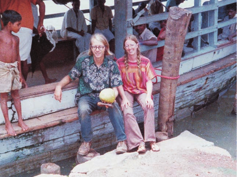
And also the theoretical part is important, especially at the very end when the algorithm finishes. But this is the easier part (in comparison). One has to exclude for example a graph (a puzzle), which can not be solved like that. [This amounts to understand that there are no constraints like in the 15 puzzle, if initially, two pieces are interchanged and where a “parity integral” must be preserved.] In the Euler refinement game this been understood already by Stephen Thomas Fisk (who was a Harvard PhD, who wrote his thesis under the advise of Gian Carlo Rota. Stephen Fisk died in 2010. Some basic ideas trace back even earlier as there is some work in 1891 by Victor Eberhard, an other remarkable German geometer who was blind (one can read about Eberhard in this excellent outreach feature article of Joseph Malkevitch). That part pretty much is explained in this paper about Eulerian edge refinements. An important theorem there is that every 2-sphere can be edge refined to become Eulerian. I assumed in 2014 that this is “obvious” but of course, it has to be proven. I prefer now to see it as a consequence of the modulo 3 lemma from the same paper as one also has to understand well what happens when refining a disk, where the boundary plays an important role. It is the game of billiards or geodesic flow which essentially tell why these things are true. I just found a picture of Stephen Fisk in the marvelous book of Burger and Starbird (“The heart of mathematics”). It shows Steve Fisk with his wife in 1975/1976 during a trip in Asia: