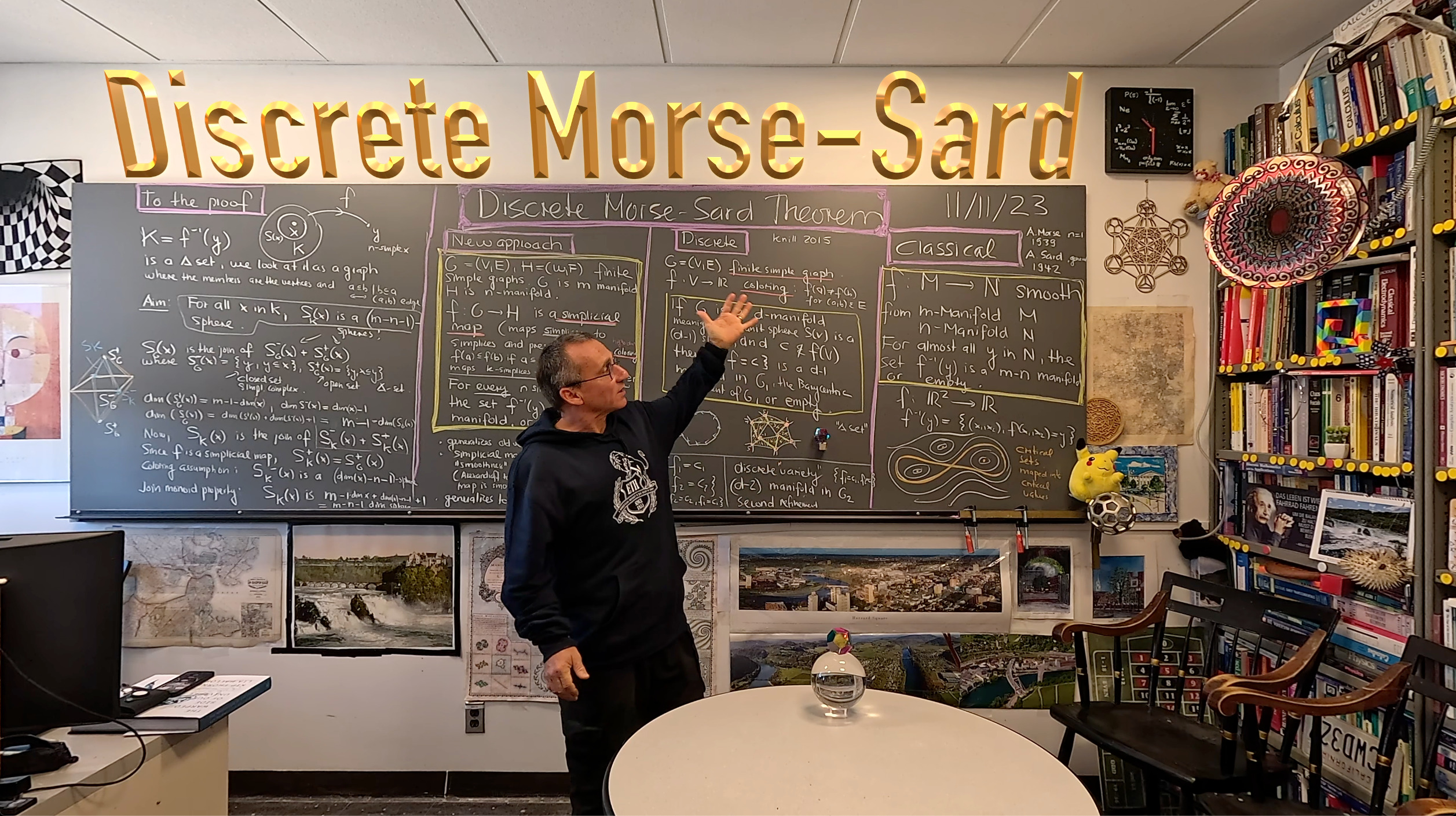
The classical Morse-Sard theorem is a very intuitive result. We encounter it in daily life. If we look at the level curves of a function like the places on earth where the temperature is constant, then for almost all temperature values, the iso-therm is either empty or a 1-dimensional manifold, meaning that it is a union of finitely many closed curves. There are rare temperature values, so called critical values, where the isotherm is a singular curve. This can happen at maxima or minima (where the level sets are points) or on curves passing through a saddle point, where the level curves typically are figure 8 type curves but they can be much more complicated in non-Morse situations like if Monkey saddle points appear where the discriminant (talked about in multi-variable calculus courses) is zero. The genius of Morse-Sard is not to look at the critical points but at critical values. If we would look at the critical points, then the result would be false: a constant function or a smooth function which is constant in some patch would have a set of critical points which have positive measure. We would need functions of more regularity like Morse functions to assure that we have finitely many critical points. But this assumption of limiting functions leads to a completely different world. Marston Morse (1890-1977) created Morse theory. [The Wikipedia article gives 1892 as birth year, but the national academies press gives 1890, the later is probably wrong as other sources give 1892, like also on his selected papers.]. It was Anthony Morse (1911-1984) who is unrelated to Marston Morse and in 1938 formulated the Morse-Sard theorem for scalar functions. Arthur Sard (1809-1980) generalized the result to maps , where M is a m-dimensional manifold and N is a n-dimensional manifold. It is a corner stones of differential topology.
What happens in the discrete, if space is quantized? It was for me mind-boggling that there is at all an analog result and especially that it is so easy. As often in discrete geometry, the analog results are by a large margin much easier than in the continuum. Examples were Gauss-Bonnet (compare the proof of Gauss-Bonnet-Chern with the almost tautological statement for general finite geometries for example where only seeing the relation between the continuum and discrete is really challenging, (but also understanding the link becomes easy when seeing Gauss-Bonnet integral geometrically)). The discrete Morse-Sard theorem can be most intuitively formulated in the frame work of finite simple graphs. Let be a coloring meaning that for . Now we define the graph $latex\{ f=c\}=(W,F)$, where the vertices W are the complete sub-graphs of G on which f changes sign. The edges are pairs of complete sub-graphs for which one is contained in the other. A graph G is a d-manifold if every unit sphere S(v) is a (d-1)-sphere. A d-manifold is a d-sphere if G-v is contractible for some v. A graph is contractible if there exists v such that both S(v) and G-v are contractible. These inductions start with the empty graph 0 being the (-1) dimensional sphere and the 1-point graph being contractible. We have used these inductive definitions (going back go Evako) for many years now and they have proven to be very, very good. One reason is that the definitions are simple. An other reason is that the inductive nature of the definitions makes proving results easy. One can delegate things to unit spheres which are again manifolds for example. Analog definitions work well also for finite abstract simplicial complexes or (the ultimate frame work) Delta sets (like for example open sets in a simplicial complex as we have seen ad nauseam here earlier in the year when working on the fusion inequality).
Theorem (Discrete Morse-Sard 2015) If G is a d-manifold and , then the graph is a (d-1)-manifold.
Proof. the graph is a sub-graph of the Barycentric refinement of G, in which all complete subgraphs are the vertices and two are connected if one is contained in the other. In order to check that we have a manifold, we have to show that the unit sphere of a vertex in is a -sphere. In the Barycentric refinement, the unit sphere in general is the join of and . (The join is the disjoint union of the two graphs enhanced with all connections between and ). Now, . Now is the boundary complex of the simplex x. It is a $(k-1)$-sphere if $x$ has dimension $k$. Now, we show that is a hyper-surface in . With that, we know that is a sphere as it is the join of two spheres. To see that is a codimension-1 sphere in , write and assume that the function $f-c$ takes negative values on and positive values on . The level surface inside the sphere is now the join of the boundary sphere of and which is a sphere of dimension . End of proof.
A side remark, to tie this in to some topics worked on earlier this year: the chromatic number of a (d-1) dimensional level surface is always d, the minimal possible color! The reason is that the dimension is a coloring. If the surface has dimension larger than 2, then the (edge) arboricity can be arbitrary large. Consequently, also the acyclic chromatic number can be arbitrary large. If the surface has dimension 2 of course, then the arboricity is either 3 or 4 as we have seen. In the 2-dimensional case, the acyclic chromatic number is 4 except in the case of prism graphs, where the acyclic chromatic number is 5. Prism graphs are very special in the class of 2-manifolds because they are non-prime in the Zykov monoid and more importantly because the set of degree 4 vertices induces an acyclic graph. Every 2-manifold which has the property that the set of degree 4 vertices (points of maximal possible curvature 1/3 in 2-manifolds) forms a cyclic graph must be the suspension of a circular graph. Prism graphs are the only 2-manifolds that are suspensions. This makes them special.
How can we formulate this more closely to the situation in the continuum, where we have a map from a dimensional manifold M to a dimensional manifold ? We want to do it in such a way that both are replaced by graphs in such a way that the set of $x$ for which $f(x) = y$ is a manifold. Warning, in the video, I improvised a bit. The topic is definitely still in the experimental phase. But we goal is to have a higher dimensional Morse-Sard which looks like the classical Morse-Sard and where does not depend on the order in which the functions are considered. I had already in 2015 tried to look at the set of all simplices in where both f and g change signs, but this was NOT a manifold in general. There must be a simple and natural way to formulate this in a way that we have for general coloring functions f,g with some non-degeneracy conditions and almost all c,g a natural way to define and get a co-dimension manifold. in the continuum, this is formulated not like algebraic geometry but in differential topology, and look at a map , from one manifold to an other.
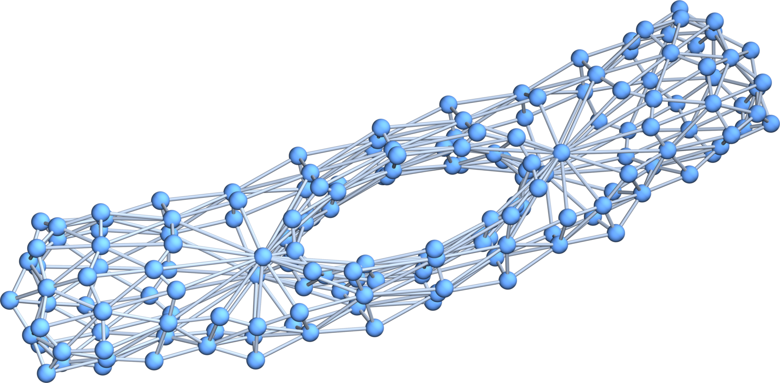
[Update of November 12, 2023: the solution to the problem discussed below is much easier. There is a frame work, where is a subgraph of the first Barycentric refinement and where it is a manifold (or empty) for almost all c,d and such that the order of f and g does not matter. (And no, it is not just taking the simplices where the both f,g change signs. This was seen already not to work in 2015. I will talk about this next time. For now, just a picture showing what one can get if one takes a 4-manifold and two random functions f,g. The result is always a 2-manifold (except of course as usual that we do not take c,d taking values which are attained on vertices such that the result is the empty graph. This is pretty cool. In this “first light” experiment, the random 2-manifold in the 4 manifold was just a 2-torus. The functions f,g were chosen at random and the host 4-manifold is a relatively small 4-sphere.]
Why were we not happy in dimension 2? Take a function g on the new graph and get within the Barycentric refinement of . This is s a different graph than on . Both graphs are sub-graphs of the second Barycentric refinement but the two graphs are different. Is there a way to get as a co-dimension 2 graph which does not depend on the order in which f,g are taken? Saturday morning, I tried an attempt and talked about it the same morning. Not yet well developed and still in an experimental phase, but here is an idea: think of as a map from the graph G to a 1-dimensional graph H, where the edges are the ranges of c, where is locally constant and so produces the same level surface. If is an edge in that 1- dimensional graph, then is the level surface . If we go one dimension higher, we want the inverse image of every 2-dimensional simplex in H to be a manifold in . As the above given proof in dimension 1 shows, we need that the stable unit sphere to be a co-dimension $2$ sphere in $S_G^-(x)$. This can be achieved, if we look at all the simplices for which change sign but where the two colors splits up the simplex into three different parts , and . Now the join of the boundary spheres of these three spheres is a co-dimension 2 sphere and the proof generalizes. The condition which we need (and which was the trouble I encountered in 2015, when looking at all simplices, where both f,g change sign) is that we need that if f,g change sign on a simplex x, that the function values f,g split the simplex into three parts. This is a local non-degeneracy condition similarly to the continuum, where we want the gradients of f and g to be non-parallel, or equivalently the Jacobian of the map from the first to the second manifold to have maximal rank. What we need is that locally, the functions f,g split a simplex into three different parts, not just two.


")

 \neq f(y)")
 \in E")
 \in F")

")

")
")


")
 = \{ y \in W, y \subset x, y \neq x\}")
 = \{ y \in W, x \subset y, y \neq x \}")
")
")
 = S_G^+(x)")
")
")
 = S_K^+(x) + S_K^-(x)")
")
")
")
")


 = dim(x)")


")


")
")
")
")