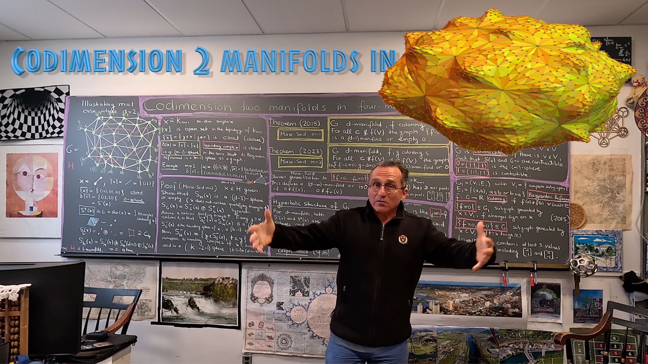
This is a continuation of the last post on discrete Sard,. We started to return after 8 years to a topic which is a classical multi-variable calculus theme especially in a Lagrange set-up. Given two functions f,g. What is the nature of the level set {f=0,g=0}? What is new since last week is that we have found (after quite many failures and wrong attempts) to find a way to make sense of {f=0,g=0} in the Barycentric refinement. In 2015, I had just known how to define {f=0} which again being a manifold can then be used to make sense of {g=0} in {f=0}. What had vexed me then is that {f=0} in {g=0} is a different graph than {g=0} in {f=0} and also the rather ugly fact that we had to lift the function f to the Barycentric refinement in order to make sense of this. Last weeks youtube video was already trying and using the proof of the theorem as a guide (it was improvisation and not good). Looking at how proofs work is essential ehen makding definition. During the construction, one should not just try out blindly with different definitions but try definitions for which a proof has a chance to work. There are many notions of “discrete manifold” but the inductvie definition used here going back to the Russian mathmatician Alexander Evako (Ivashchenko) is the good one. Its recursive definition allows to prove things and delegate notions from dimension d to unit spheres which are manifolds of dimension d-1. Also “beauty” is a guidance. As simpler the definitions, the better. I had tried in 2015 already to look in the second Barycentric refinement directly for conditions to impose to make sense of the codimension 2 object {f=0,g=0} which does not depend on the order. Nothing worked until last week. Of course (having taught Lagrange method for more than 35 years now first as an undergraduate course assistant at ETH and teaching it since), I’m had been very much interested in getting Lagrange to work in a completely discrete setting and now finally, I start to see how it works on rather arbitrary networks. Of course, it will be nicer for manifolds as also in the continuum, the Lagrange theory is best done on manifolds on not on arbitrary topological spaces.
Here is the definition. Given two colorings f,g which do not attain the value 0, define {f=0,g=0} as the sub-graph of the Barycentric refinement generated by all simplices x on which the vector (sign(f),sign(g)) takes at least 3 values including the values (-1,1),(1,-1). That’s it! So, we want both f and g change sign on x as well as having some non-degeneracy condition assuring that the “gradients are not parallel” which is encoded in that the sign function includes a triangle. This generalizes the case f=0, were we just wanted that sign(f) contains at least the two values 1 and -1. In higher dimensions, this works in the the same way. Given 3 functions for example, we want sign(f,g,h) to take values (-1,1,1),(1,-1,1) and (1,1,-1) and take at least 4 different values. This produces then a discrete Morse-Sard theorem telling that for a 
")
Why do I think being able to remain in the first Barycentric refinement is a big deal? It is practical. Working in second Barycentric refinements already is terrible also because they are rather large. The smallest 4-manifold of all is the 4-cross polytop, a 4-dimensional sphere. It has 10 vertices, 40 edges, 80 triangles, 80 chambers and 32 hyperchambers and the figure below shows this 4-manifold on 10 nodes. The first Barycentric refinement is manageable. It has 242 vertices, 2640 edges, 8160 triangles, 9600 chambers and 3840 hyperchambers. The second Barycentric refinement makes you or your computer sweat: it has the f-vector (24482, 303840, 970560, 1152000, 460800) meaning that we have to deal with already half a million of 4 dimensional chambers. And note that we started with the smallest possible 4-manifold of all. It is a big deal if we can make sense of {f=0,g=0} in the first Barycentric refinement. I myself am a very down to earth mathematician who wants to work with stuff not just theoretize about it. So, if we have a construction, I want to have examples with which I can work with and which I can see, even if it requires a computer to do so. I would love for example to look at examples of surfaces {f=0,g=0} on homology spheres, which are 3-manifolds which have the same homology groups than the sphere but are not equivalent as the fundamental group is different. With the new approach this is now possible. There is a homology sphere graph with f-vector (568, 3688, 6240, 3120) for example. Its Barycentric refinement has the f-vector (13616, 88496, 149760, 74880) but its second Barycentric refinement would have f-vector (326752, 2123872, 3594240, 1797120) which is too tough to work with. I would have to write specialized C-programs to be able to work with that. Computer algebra systems are too slow for that. I can however work in the first Barycentric refinement.
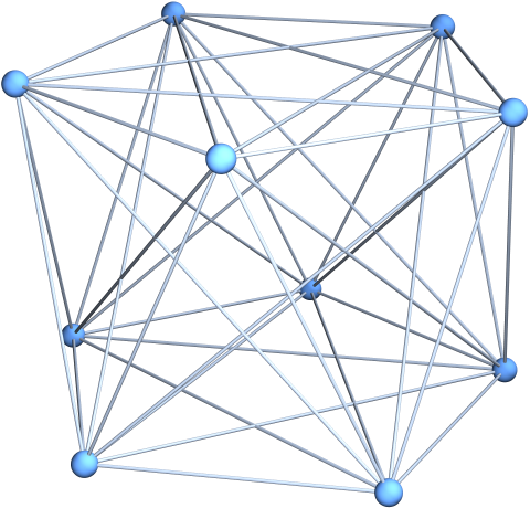
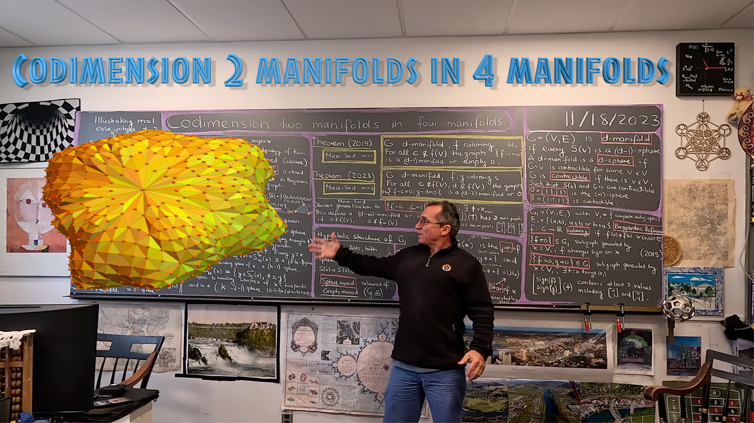
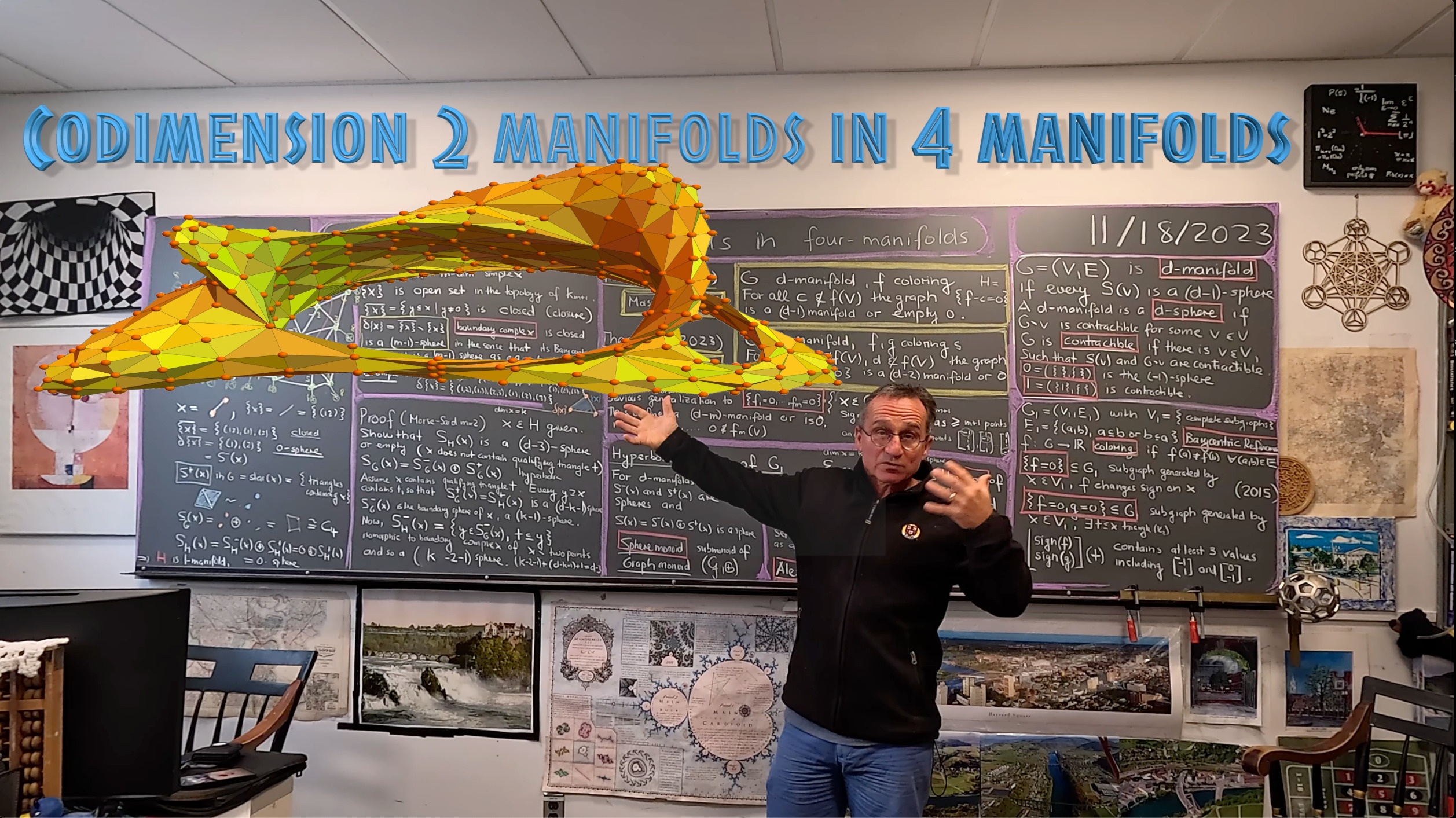
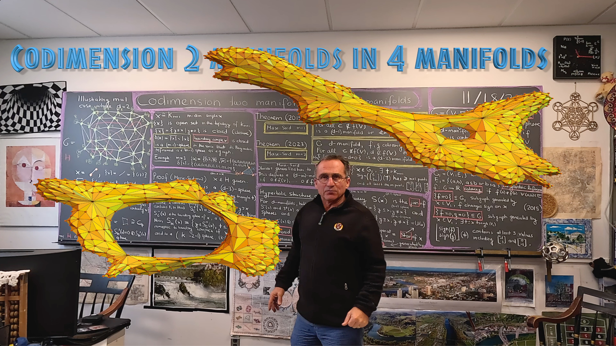
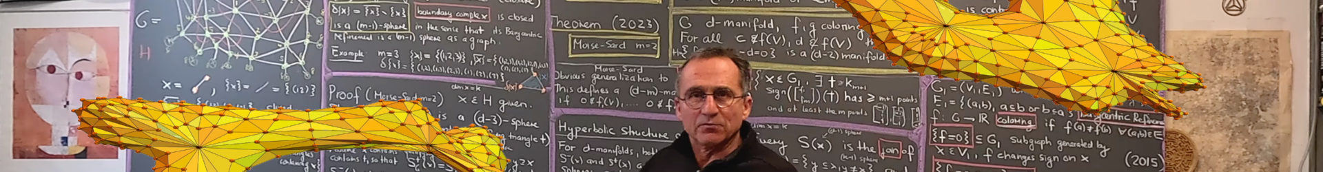
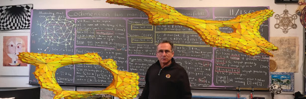
By the way, the smallest 4-sphere is the join of an octahedron graph O with a cyclic graph C4. Every unit sphere is a 3-sphere (the join of two C4). Every unit sphere in a unit sphere is an octahedron. The Gauss-Bonnet-Chern curvatures of this 4-manifold is constant 1/5. There are 10 vertices so Gauss Bonnet adds to 2 as all even dimensional spheres have. The Betti numbers are (1,0,0,0,1). Since the manifold is orientable there is Poincare duality. We also will work with 4-tori which is a Calabi-Yau manifold and can be seen at Porter square. The torus example shows also where we are going. The manifold is also a Kaehler manifold and the level surface {f=0,g=0} can be seen as the level surface of a complex function f+ig, a complex curve. Now, in the discrete, we can realize rather fancy objects with a few nodes! We might get into this next time. In the examples shown in the movie, I would take as a host graph a slightly larger 4-sphere like the join of an octahedron with a larger cyclic graph or the join of an icosahedron with a cyclic graph. In the last picture (showing a 2-sphere), I took the join of C4 with a pentakis dodecahedron (which is a 2-sphere). Taking a larger Catalan solid like the disdyakis triacontahedron or Barycentric refinements or edge refined versions allows to produce a rich variety of 4-spheres.
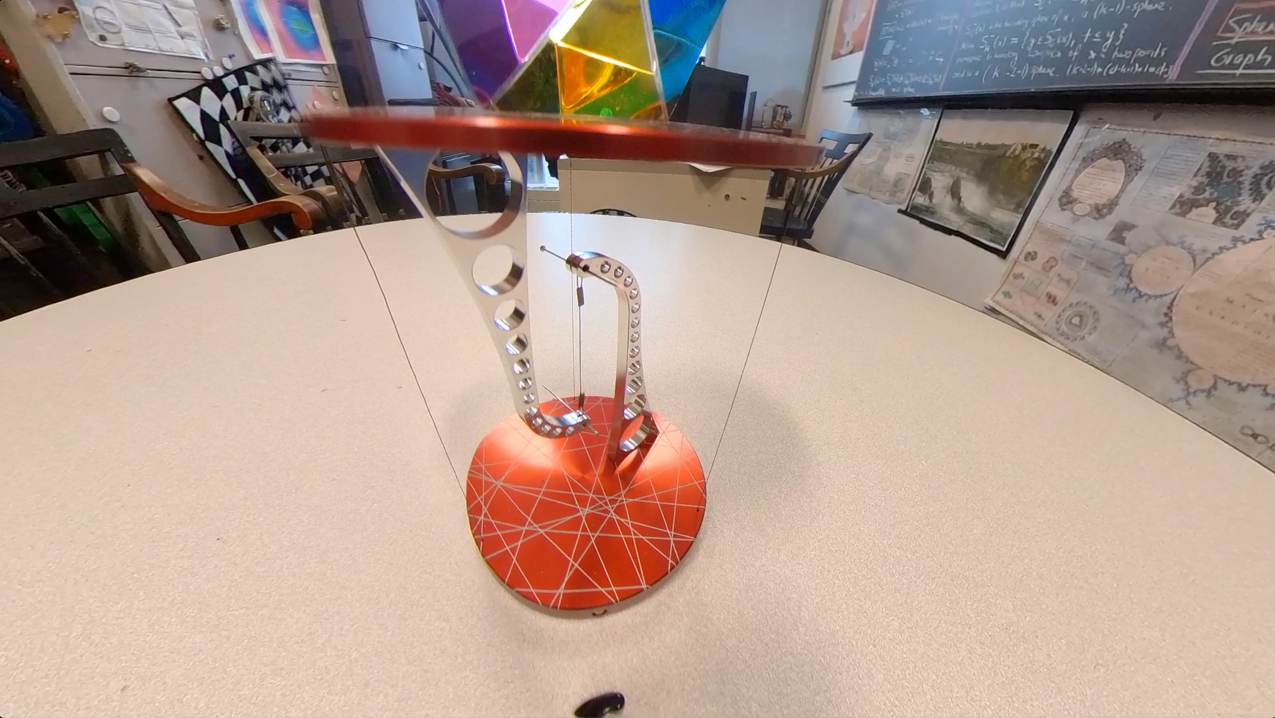
The manifolds were generated in Mathematica as level surfaces in small 4-spheres (taking random function f,g). I had just obtained the Tensegrity model yesterday which appears in the intro part of the movie. The stable configuration of this object is a natural critical point of a potential function f on a 4-manifold (3 translations and one twist rotation parameter). If we constrain on g=0, where g is the angle. then we have a Lagrange constraint situation and deal with a critical point of a function on a 3-manifold. This is what are doing here in the discrete. Multivariable calculus and much of differential geometry almost collapses to tautologies in the discrete. This can be seen when looking at theorems like Gauss-Bonnet or Poincare-Hopf or the Brower Lefshetz fixed point theorem. When I taught Math 22 (in the good old times when it was still possible to teach an original math course at Harvard). I would dedicate 2 proof lectures to discrete calculus which means covering Green,Stokes and Gauss in a graph theoretical frame work. See the easter bunny lecture. More than 10 years ago, in the spring of 2013, I presented single variable calculus including the fundamental theorem of calculus and Taylor’s theorem in 20×20 seconds. See “If Archimedes would have known functions”. See the text to this talk. I took pride then in to be able to cram the essence of single variable calculus into one page and the essence of multi-variable calculus into one page. This was possible because one does in the discrete not have to be distracted by notions like limit. If you put yourself into the mind of the creator of the word who has to decide in a split second (like the Planck time