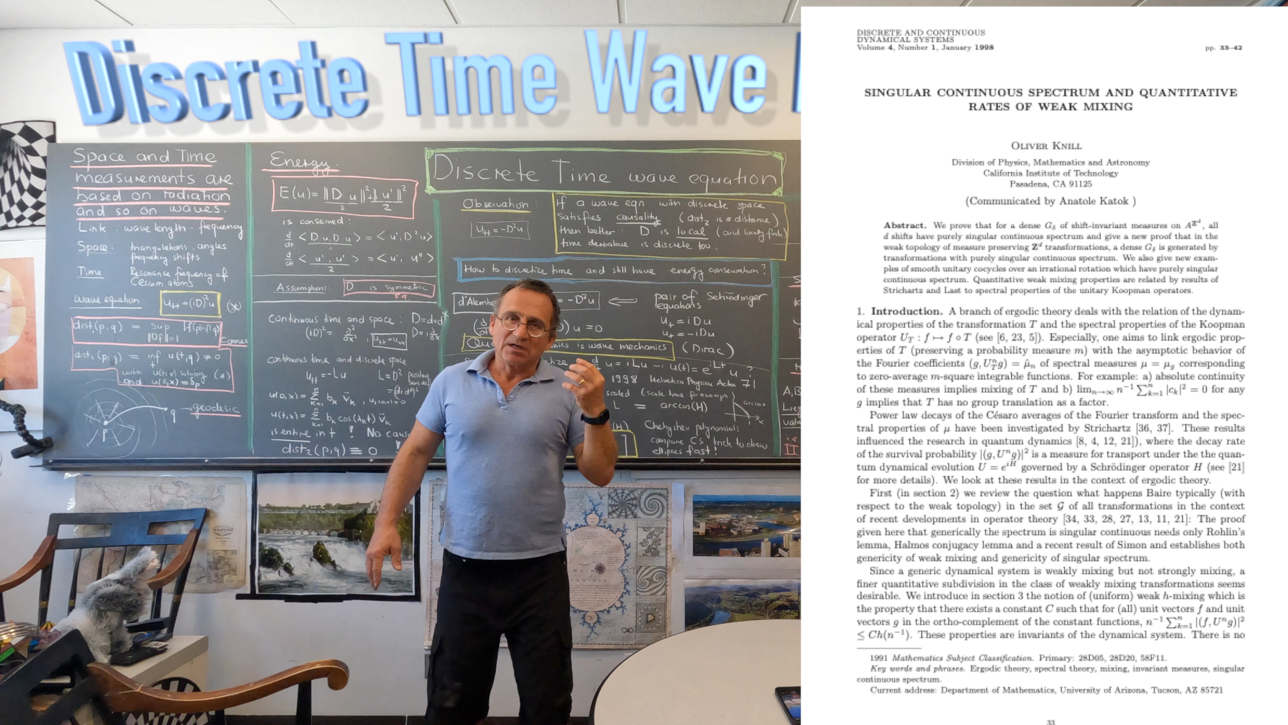
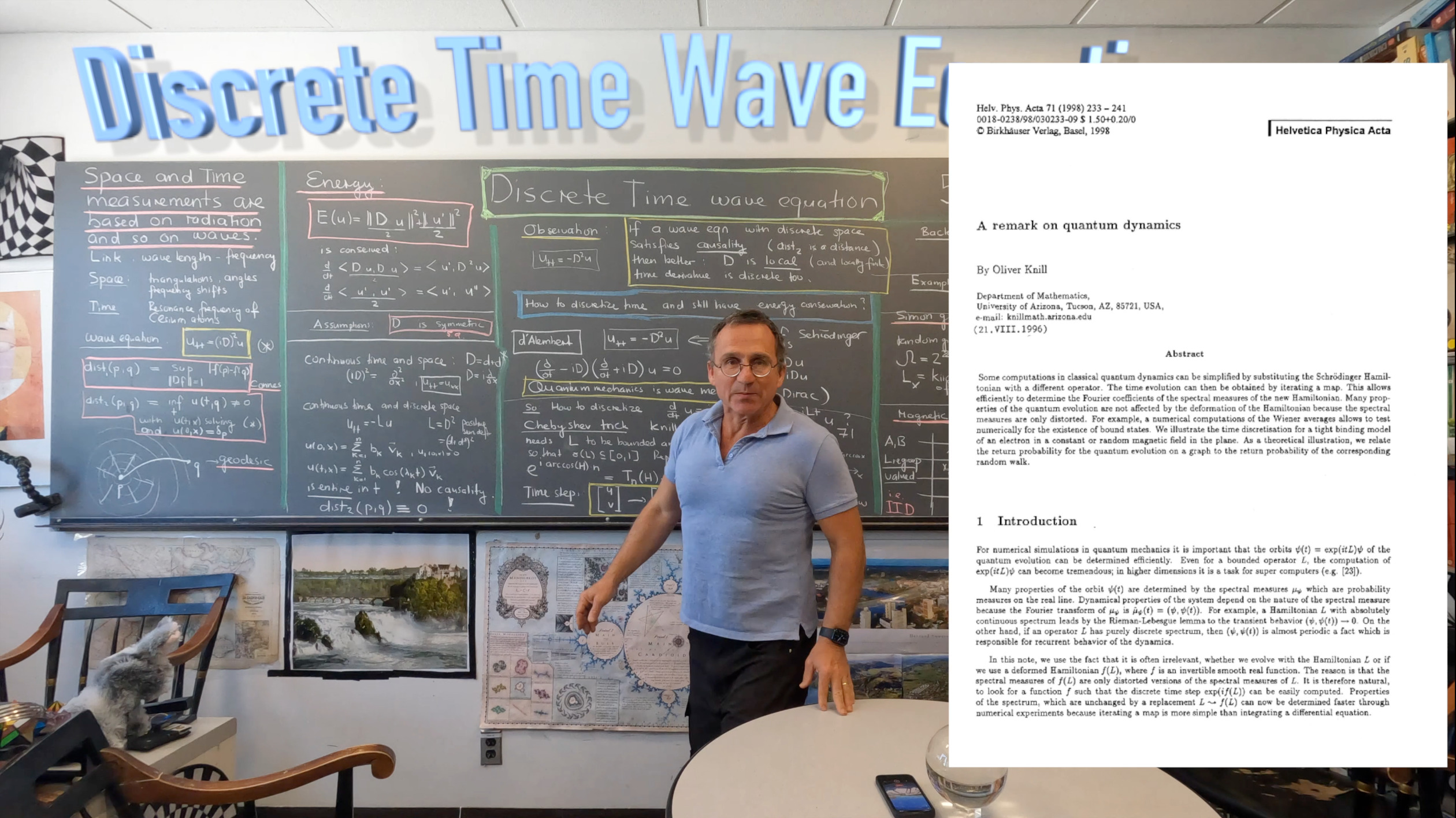
It is a simple but interesting fact that if we look at a wave equation with discrete space, we also need discrete time provided we want causality, a property which every wave equation should have. The reason is that the solution equation in a causal locally finite geometry is an explicit analytic solution in terms of eigenvalues and eigenfunction of finite matrices and in particular provides entire (analytic in ) solutions in time. An analytic function can not be constant for some time interval as otherwise, it would be constant. So, if the universe would have locally finite discrete space structure and we started a wave 10 light years away, we still could see notice a change of the amplitude of the wave here, even after one second. Of course, this change is ridiculously small and any physicist would call it zero, but it is not zero. The solution is of course to discretize time also. Of course, we need the Hamiltonian property preserved. I used once such a numerical scheme here and also made some pictures like this from 1998. An X-window C program would actually do it in real time. The discretisation is very simple. If L is the operator, scale it so that its spectrum is in [0,1], then use the iteration which is conjugated to a unitary evolution. In that paper, I had used it to investigate the spectral properties of the magnetic operator on , where $A u(n,m) = a(n,m) u(n+1,m)$ and and where are IID random variables taking values in . This is a lattice gauge field setup. The experiments indicated that there is no point spectrum. I expected the spectrum to be singular continuous. This can be investigated by computing the Fourier coefficients of the spectral measures and see how they decay. By Wiener’s theorem, the Cesaro average goes to zero if and only if there are no eigenvalues.
By the way, there is an interesting story the magnetic operators investigated in my Quantum dynamics paper: the general problem is that if B(n,m) are random variables on the plaquettes (with the same distribution but not necessarily independent) but with some distribution. Can we find gauge fields (functions a(n,m), b(n,m) as given in the problem) such that B(n,m) is the discrete curl meaning the line integral along the boundary of the plaquette. In one dimensions, the answer is no in general. Every stochastic process with random variables can be realized as , where is a fixed function and a measure preserving transformation. But not every random variable can be written as for an other random variable! There are cohomological constraints. The higher cohomologies however are trivial. Especially, every magnetic field stochastic process (with 2 dimensional time) can be realized through gauge potentials. In the case of IID random variables with uniform distribution, the a(n,m), b(n,m) also can be chosen to be IID random variables. Of course the spectral question is interesting also in other situations like if a(n,m) and b(n,m) would be almost periodic sequences. The story of the Almost Matthieu operator indicates that one would have singular continuous spectrum there, at least generically. I once used Barry Simon’s Wonderland theorem to give new proofs in ergodic theory that a generic measure preserving transformation has singular continuous spectrum and that a generic invariant measure of the shift operator leads to a dynamical system with singular continuous spectrum.


 \to (2Lx-y,x)")

")
 = b(n,m) u(n,m+1)")
, b(n,m)")
 = \{ z \in \mathbb{C}, |z|=1 \}")
 = g(T^nx)")


 - X")