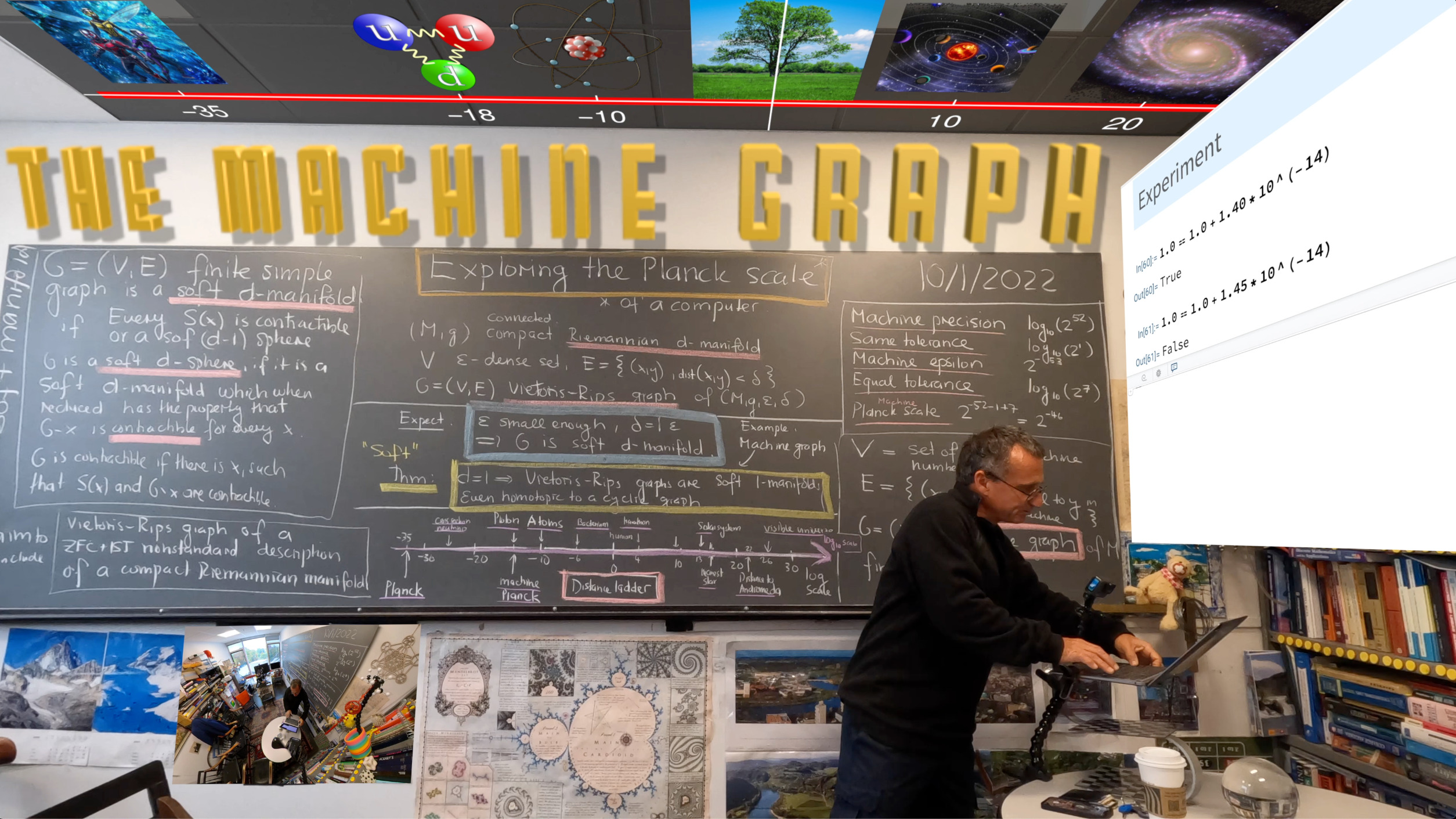
The Planck Scale on a Computer
The physical Planck scale of 
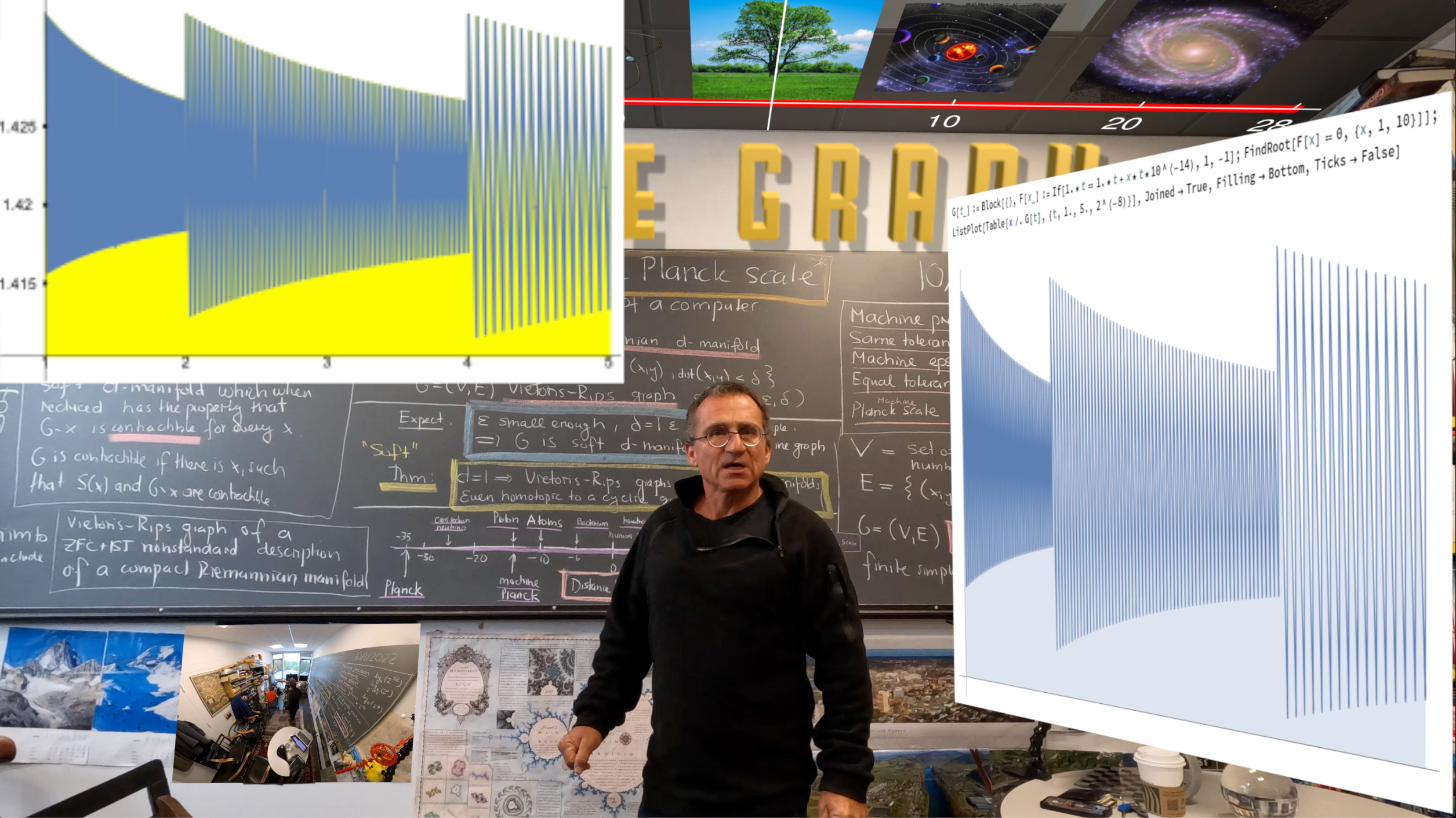
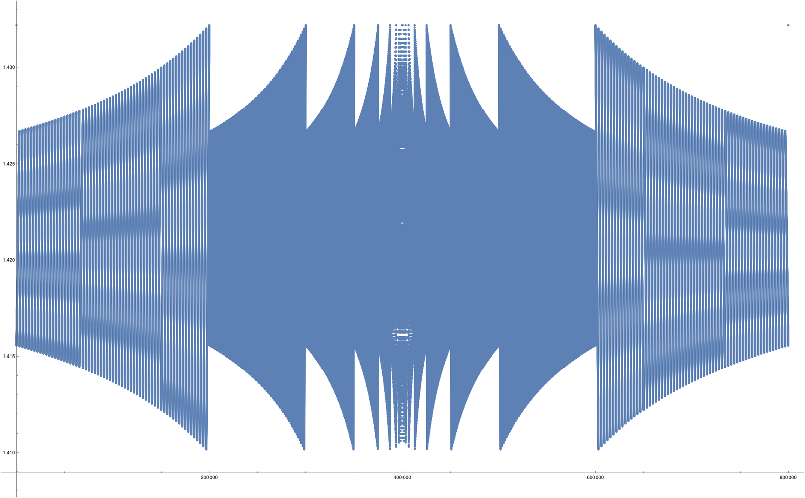
1.0+1.4*10^(-14) ==1.0 gives us True but 1.0+1.4*10^(-14) ===1.0 gives us False. The threshold h, where 1.0+h*10^(-14) ==1.0 stops being True is the analog of a machine Planck scale. We can explore this numerically F[x_]:=If[1.0==1.0+x/10^14,1,-1];FindRoot[F[x]==0.,{x,1,1.5}] and the answer is h(1.0) =1.43219… This number is determined by machine precision, same-tolerance and equal-tolerance parameters and close to 2^(-46) which is about 1.42109*10^(-14). What is the exact value? In order to see this, we need to see how this threshold changes with the base point. G[t_] := Module[{}, F[x_] := If[1.0t == 1.0t + x*t/10^14, 1, -1]; FindRoot[F[x] == 0., {x, 1, 1.5}]]; ListPlot[Table[x /. G[t], {t, -4.0, 4.0, 0.00001}], PlotRange -> All]
The Machine Graph of an Interval
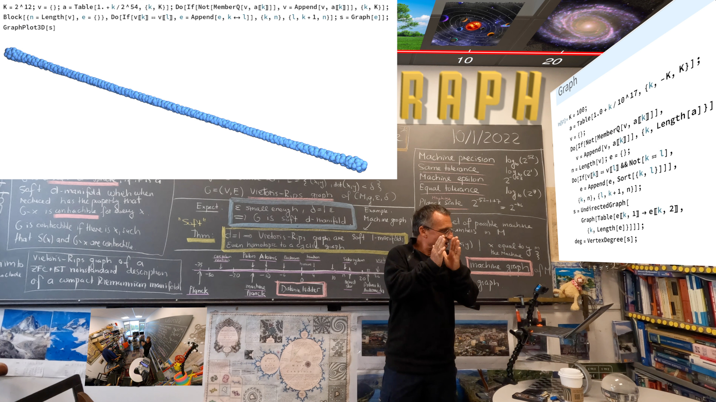
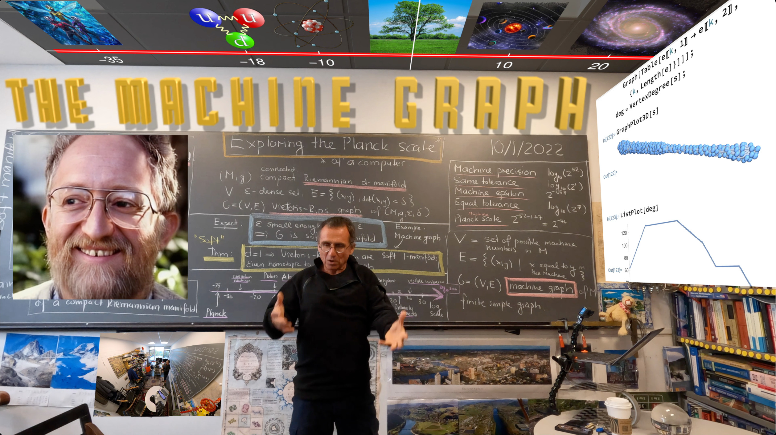
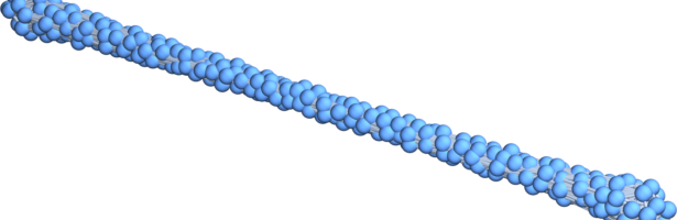
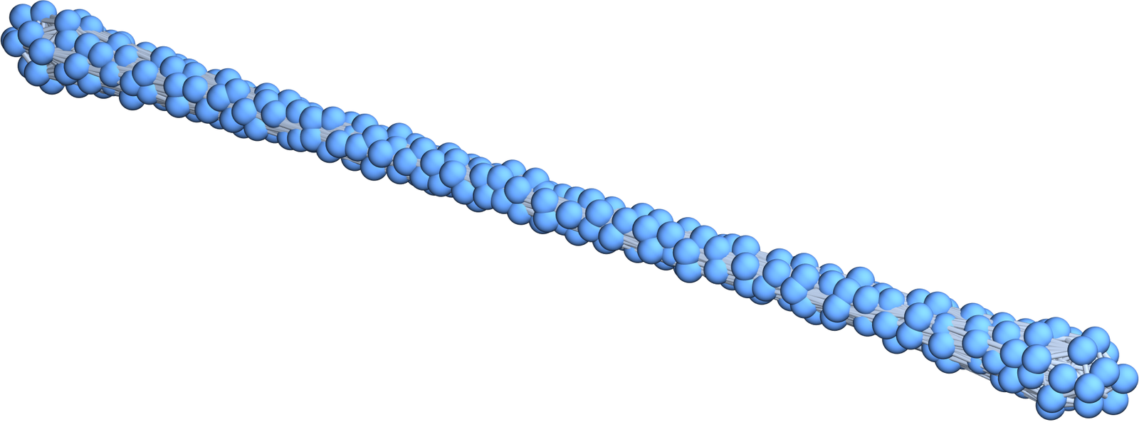
We can now look at all the numbers in the computer contained in some interval and make a list of those that are not the same then connect two if the are equal. This produces a graph, a machine graph. Here is how we can produce it. We take for example a tiny interval from 0.14-2^(-43) to 0.14+2^(-43). Here is the code: K=2^12;v={};a=Table[0.14+0.14*k/2^55,{k,-K,K}];Do[ If[Not[MemberQ[v,a[[k]]]],v=Append[v,a[[k]]]],{k,K}]; n=Length[v];e={};Do[ If[v[[k]]==v[[l]],e=Append[e,k<->l]],{k,n},{l,k+1, n}]; S=GraphPlot3D[Graph[e]]. It produced the picture below. It is an example of a Vietoris-Ribs graph. In the machine graph, every unit sphere has a few dozen elements (the maximum is 69 in our particular case and every unit sphere is contractible). The maximal dimension is 69. Still, it has a one-dimensional topology built in. If we remove points (not at the boundary) which are contractible until we can no more do that, we end up with a linear path graph. The Euler characteristic of the graph is 1. The actual dimension only reveals if melting away contractible parts away from the boundary. [Below are again the definitions of a soft manifold. It was important to look at manifolds without boundary. Otherwise the definitions do not work well. The Vietoris-Rips graph of an interval and in particular the machine graph is homotopic to a point and not a soft manifold. The wheel graph is a discrete hard manifold with boundary but not a soft manifold because we can melt away the boundary to get to a point. The wheel graph is not a soft 0-manifold because there is a unit sphere in it which is a 1-sphere. If we identify left and right point of the machine graph, we get a soft manifold in that sense.]
Nonstandard Notions
In nonstandard analysis thenotion of infinitesimals appears. The notions have been pioneered by mathematicians like Leibniz or Cauchy already. And this has been axiomatized in various frame works. I grew up in the frame work of IST, which is a consistent extension of ZFC and could see an entire calculus course built up with these notions taught by Hans Laeuchli, a logician, who taught that course at ETHZ (I have notes still here) and who also had been my calculus teacher in Analysis I and Analysis II for the first two semesters at ETHZ. It had been was an eye-opener to see that compact topological spaces behave like finite sets. Indeed, the proof of Bolzano’s theorem that a real valued continuous function on a compact set X has a maximum is just proven by the fact that a function on a finite set has a maximum. Now, if we look at the points which a computer can represent of an interval [a,b], then this is a finite set. There is a smallest h(x) (as just explored) for which x and x+h(x) are considered equal (even so they are not the same). This allows us to play with already built-in structures and simulate non-standard notions. Here is an example: there are non-zero numbers h on a computer such that h^2=0. We can then use these infinitesimals to compute derivatives.h=1.02^(-24); {1.0+h ==1.0,1.0+h*h==1.0} shows that h*h is too small. Now we can take derivatives d[f_,x_]:=(f[x+h]-f[x-h])/(2h); u=d[Sin,1.0]-Cos[1.0];1.0 + u*u == 1.0. We see that the computer identifies the discrete derivative with the real derivative. No limits involved at all. Everything is finite. Everything is already built into a machine and determined by parameters like machine precision, equal -threshold or same-threshold parameters.
Vietoris-Rips Theme
On can look not only at intervals but rather arbitrary topological spaces. It is not a bit deal to focus on compact topological spaces M. [If a space M is non-compact, just compactify in some way. The choice of compactification depends on the mathematics. In most cases a 1-point compactification suffices. In projective geometry one has a more sophisticated notion as one places a sphere at infinity. Now one can deal with a finite set V such that all points are infinitesimally close to V. (One can also just fix an 


<\delta")
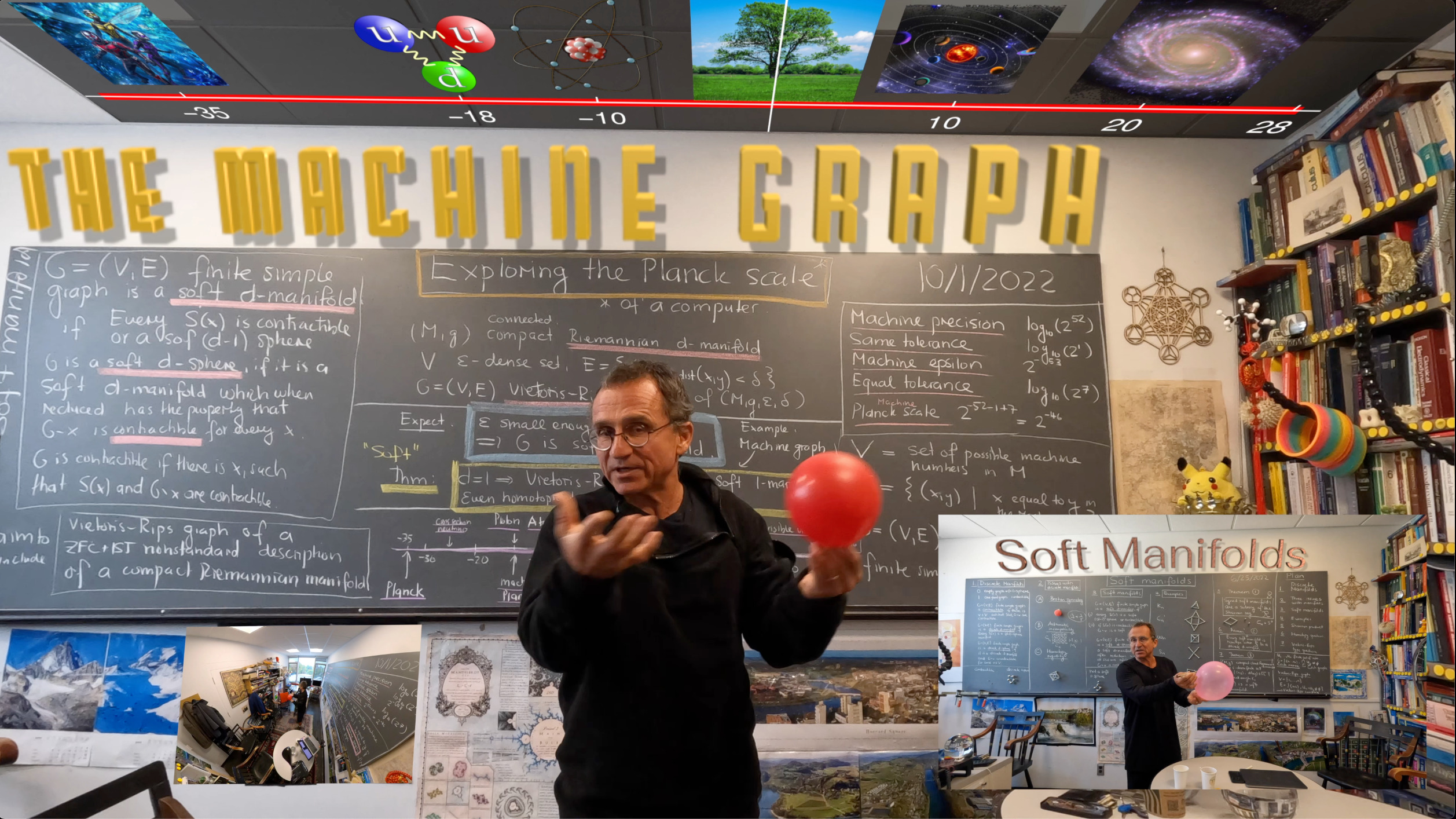
Soft Manifolds
Motivated from graph complements of circular graphs, the notion of soft manifold appeared.(For videos, see here or here). Three theorems still need to be proven: 1) Vietoris-Rips graphs of compact closed Riemannian manifolds are soft manifolds, 2) Shannon products of soft manifolds are soft manifoldsand 3) soft manifolds allow homotopy reduction to hard manifolds This still needs work. In the one-dimensional case, the proofs of 1)and 3) is an exercise sketched in the video. In general, the idea is to show the Shannon product case 2) first, then use this to verify 1) and 3) as locally, we can see a manifold as a products of one dimensional soft manifolds similarly as manifolds are locally Euclidean, locally the Cartesian product of one dimensional spaces.
Here are again the recursive definitions: a soft d-manifold is a finite simple graph such that every unit sphere is either contractible or a soft (d-1)-sphere. A soft d-sphere is a soft d-manifold so that after some homotopy reduction, (remove a point x for which both G-x and S(x) are contractible), every unit sphere is a soft (d-1)-sphere. A hard d-manifold is a finite simple graph such that every unit sphere is a hard (d-1)-sphere. A hard d-sphere is a hard d-manifold such that G-x is contractible for every vertex x. A graph is contractible if S(x) and G-x are both contractible for some x. The 1-point graph (the unit 1 in the Shannon ring) is declared to be contractible. The empty graph (the additive zero in the Shannon ring) is declared to be a a (-1)-sphere.
Another motivation to enlarge the class of hard manifolds was that the later have usually very rigid symmetry. Soft manifolds can in a non-standard setting have the property that the admit every standard symmetry of a continuum Lie group symmetry. Think about it as such. Take a finite set of points you care about (for example which you are able to measure) and take a finite set of symmetries T you care about (for example the finite set of operations you can ever perform), then take the union of all T(x) where x is in the finite set of points and T is in the finite set of operations. There is now larger (still finite) set which has the property that for all points and all transformations you care about, also the image is in the set.