Exponential Patch

Given a finite abstract simplicial complex G that is a q-manifold, we consider a k-simplex y in an oriented maximal simplex x as an element in the Grassmannian G(k,q). Of course we are in finite geometry and have no vector spaces but a maximal simplex serves as a q-dimensional frame and a k-simplex can be considered as the analog of k-dimensional subspace. Similarly as in the continuum, where an element in the Grassmannian of the tangent space of a point p in a Riemannian manifold M, defines a k-dimensional geodesic sheet obtained by running all geodesics within the subspace, we want to get in the discrete a k-dimensional discrete manifold passing through that point in the Grassmannian. In the case k=1, this is just the geodesic. In the two dimensional case, this is a geodesic sheet that we have used last year to define sectional curvature. Below is some code which generates the local patches. As written, it first defines a 5 dimensional simplicial complex, (a 5-sphere), then chooses a random oriented facet x, then a random k=2 simplex y in x, then displays the patch it generates as I describe it in the video. Furthermore, the curvature is printed. It is a sectional curvature. In the case of the manifold at hand, all sectional curvatures are positive.

What is new and what still needs to be worked out that is that I had thought last year that the pair (x,y) would define a sub-manifold in the frame bundle of G. This is not the case, we need the analog of the Grassmanian G(k,q) and look at pairs (x,y) as it could happen that we move along the manifold and get back to x with the same orientation but that y has shifted. The code below does only compute the local version (which is enough for sectional curvature). We would like to see however what kind of manifolds do appear, especially when considering higher dimensional manifolds. But this also needs a result. We have to verify that we can transport the Grassmanian along. At the moment, I do not see any problem. But is often a famous last word. One of the warning signs is that in the continuum, if we look at a geodesic sheet (it exists) and chose an other point on the sheet, then the sheet starting at that point is not the same than the original sheet. An other thing we want to check and to be true is that in a 2 dimensional situation we have 6 geodesics on the surface. In a 3-dimensional pack, we would have all 24 oriented geodesics through x are on the sheet. An other thing we want to check is whether if we have a 2 dimensional sheet in a 3 dimensional complex, then what the nature of the boundary of this sheet is if we look at the union of all its simplices as defining a solid. In the case of geodesics, this boundary consisted of a flat torus.

Generate[A_]:=If[A=={},A,Sort[Delete[Union[Sort[Flatten[Map[Subsets,Map[Sort,A]],1]]],1]]];
Whitney[s_] :=Map[Sort,Generate[FindClique[s,Infinity,All]]];
Facets[G_]  :=Select[G,(Length[#]==Max[Map[Length,G]]  ) &];
OpenStar[G_,x_]:=Select[G,SubsetQ[#,x]&];      Stable[G_,x_]:=Complement[OpenStar[G,x],{x}];
Mirror[G_,y_]:=Module[{U=Stable[G,y]},Table[First[Complement[U[[j]],y]],{j,Length[U]}]];
T[G_,x_]:=Append[z=Delete[x,1];z,First[Append[Complement[Mirror[G,Sort[z]],{x[[1]]}],x[[1]]]]];
Bundle[G_]  :=Module[{f=Facets[G]},Flatten[Table[Permutations[f[[k]]],{k,Length[f]}],1]];
Dual[H_]:=Module[{e={},n=Length[H]},Do[If[Length[Intersection[H[[k]],H[[l]]]]==Length[H[[1]]]-1,
    e=Append[e,H[[k]]->H[[l]]]],{k,n},{l,k+1,n}]; UndirectedGraph[Graph[e]]];
s = GraphJoin[GraphJoin[CycleGraph[11], CycleGraph[5]], CycleGraph[4]]; k=2;
G = Whitney[s];   F=Facets[G];   q=Length[First[F]]-1;
x=RandomChoice[F];                      y=RandomChoice[Select[Generate[{x}],Length[#]==k+1 &]];
a=Select[Generate[{y}],Length[#]==k &]; b=Table[Complement[x,a[[k]]],{k,Length[a]}];            
s=Table[Stable[G,b[[m]]],{m,Length[b]}]; S=Table[Select[s[[m]],Length[#]==q+1 &],{m,Length[s]}];
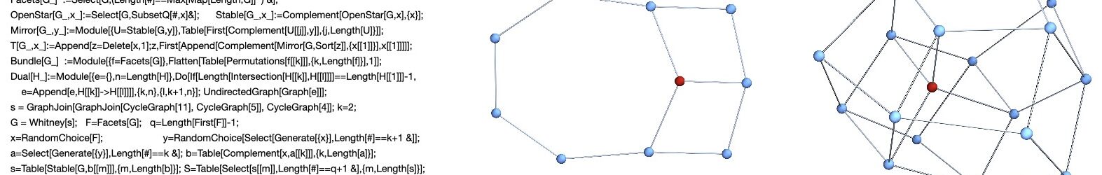
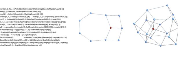
ss=Dual[Flatten[S,1]];  GraphPlot3D[HighlightGraph[ss, {x}]]
Print[Total[1/Map[Length, S]] - 1/2];