Critical points

Assume f is a continuous function of one real variable. Lets call a point p a critical point of f if Df(p)=0 where Df(x) = f(x+1)-f(x) is the discrete derivative of f. As in classical calculus, a point p is called a local maximum of f, if there exists an open neighborhood U of a, such that for all x in U. We define local minimum similarly. We can now state the following theorem:

Theorem: If a continuous function has a critical point p, then it has a local maximum or local minimum in the open interval .

The proof is a simple consequence of the extreme value theorem. If f is smooth, then by the intermediate value theorem there is even a point in the open interval where we have a classical critical point.

Despite its offending simplicity, the theorem shows that with the right definitions, a theorem can become elegant. This theorem is of course false in classical calculus: the function which has a critical point at 0 but no local maximum there.

The above theorem is not only unconditionally true, it is also more robust than the classical result. The only non-robust case is if f has a critical point at p and is constant between p and p+1. In the classical setup, any horizontal inflection point is structurally unstable. The smallest perturbation of the function can either make it monotone like with where a is arbitrarily small and positive or can produce two local extrema when a is arbitrarily small but negative.

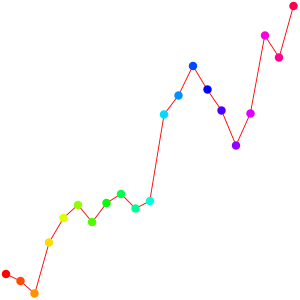
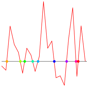
What about practical uses of this theorem? Lets go back to our DJI data which we have already seen in the Taylor page.

To the left we see the Dow Jones data from the last 20 days taken on January 15, 2011. The data define a continuous function f(x) which is the linear interpolation between the data points. To the right we have plotted the derivative f'(x) = D f(x) = f(x+1)-f(x) and also marked the critical points. If you compare with the left graph you see that it spotted the extrema pretty well. We could use classical calculus to achieve this too: interpolate the data with smooth functions like polynomials or splines then find the roots. But there is no doubt that the detour over classical calculus is more costly. Working directly with the discrete data is faster, even the root finding is trivial.

I want to add a remark about the pedagogy when dealing with critical points. Traditionally, in most textbooks, critical points include points where the function is not defined or where the derivative of the function is not defined. This produces some advantages like that it enlarges the class of points where extrema can occur. The graph of the function f(x) = |x| for example has no tangent at 0, but 0 is still a minimum. But making the notion of critical point complicated has also severe disadvantages. A student really has no clue any more what a critical point is because the class of singularities can be complicated, especially in higher dimensions. I believe that basic definitions and important theorems have to be simple.This can be done in classical calculus – whether single or multivariable- by delegating points where the function or a derivative is not defined out of the domain of the function. Points where derivatives do not exist or worse where the function is not defined need special attention anyway. A whole field of analysis called catastrophe theory illustrates this. Therefore, I prefer to restrict the notion of critical point in classical calculus to points in the domain where the derivative is zero.

At last, I would like to point out that the above result also illustrates that “calculus without limits” is not a replacement of classical calculus. It stands on the shoulders of it. While it could historically well have been developed a thousand years before classical calculus, it only is appreciated fully with the knowledge and the (pedagogical) shortcomings of the later.