Define , which leads to polynomials like
. For a function on the integers define the derivative
. Denote by
the n’th derivative. For example,
.
Theorem:The Taylor formula
holds now for all
This Taylor theorem is called Gregory-Newton interpolation formula and is useful for data fitting, since one can construct the polynomial by hand. If the function if has integer values, then the Taylor coefficients are rational. For finitely many data, we do not need an infinite sum and the Taylor series is finite.
For the proof note that the polynomials form a basis in the space of polynomials of degree n. Now all you hav to check is that
and are language wise equivalent to standard calculus. We could define a continuous function to be “real analytic” if there exists a constant r such that
. Then the Taylor series would have a finite radius of convergence at every point.
What is it useful for? The Taylor series allows you to fit data with much less effort than standard fitting methods. If you have data given as a sequence of numbers, you can compute differences at the first data point and find so a polynomial which passes. If you compute n differences at the origin, you can get a fit through n+1 points. Of course, this can also be achieved using linear algebra but it is complexity wise faster to compute the Taylor series. Matrix inversion needs about
operations while the Taylor series can be done with less than
operations. It can actually be done by hand for a dozen data points by hand while inverting a 12×12 matrix by hand is no trifle. [ Remark. To be fair, our knowledge of Linear algebra is good enough that we could in this case probably find a numerical method suited for this data fitting problem equating the one from the Taylor formula, but it would be a hack.]
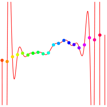
Here is an example where 22 DJI data points were taken on January 15th. You see that f(0)=11499.3 and f'(0)=-7.34, f”(0)=-6.44. The fact that the Taylor coefficients
grow fast is an indication that the data have large fluctuations.
Does the Taylor series provide us with any insight which we can not obtain otherwise?
Maybe. The radius of convergence of the Taylor series for example could give an indication on how “smooth” the data are. For polynomials or more generally for functions which are entire in the classical sense the radius of convergence is infinite too. A concrete problem would be to find a relation between the fractal dimension of the graph of f and the radius of convergence of the Taylor series. How does the radius of convergence depend on the Planck constant h, which has been chosen to be 1 in our case? These questions are probably not so easy to answer. Note that any 1 periodic function has a trivial Taylor expansion. On the level of the constant 1, nothing interesting happens with the function.
I finish this post with a few remarks. As the history of calculus has shown, notation is crucial for a theory. Newton used clumsy notation and used strange terms which did not survive. The more elegant calculus setup of Leibniz was pedagogically more successful.
The Taylor theorem stated above is so simple that in principle it could have been found by early Babylonian, Greek, Chinese or Indian mathematicians. It only involves differences and sums and can even be formulated without algebra. It especially does not involve any limits, a concept which is the stumbling block for many students to learn calculus. It also explains the classical Taylor theorem very well because it is the same theorem. With the right notation, the mathematical structures have merged. Historically, Gregory used it to derive the Taylor theorem, 44 years before Taylor (see Stillwell, “Mathematics and its History”). The difference Df(x) = f(x+1)-f(x)can be replaced of course with Df(x) = (f(x+h)-f(x))/h as Newton did and as also used in the book of Victor Kac and Pokman Cheung. But it does not make any difference. Just think of units of Angstrom, the size of a water molecule and the above Taylor theorem is so close to the classical one that one could work with it. But we do not need to dive into the quantum world at all. The theorem is already useful for analyzing data sets, as just shown.

