A Gauss-Bonnet connection - Quantum Calculus

The Green function story becomes more exciting as differential geometry has come in. We have seen that if G is a finite abstract simplicial complex, and G’ the connection graph with adjacency matrix A, then (1+A) is unimodular by the unimodularity theorem. (See also the entry on this blog). Having seen that the Green function values $g(x,y) = (1+A)^{-1}_{xy}$ are invariant under Barycentric refinements, we proved then a Green unit sphere formula $g(x,x) = 1-\chi(S(x))$ . In the sphere geometry paper it is also shown that the set of Poincaré-Hopf indices $i(x)=1-\chi(S(x))$ is a combinatorial invariant, meaning that it the sphere spectrum $\{ i(x) \; | \; x \in V' \}$ does not change when doing Barycentric refinements.

Yesterday, on February 16, an experiment showed the following “anomaly”,[not a weak signal like in the LHC, but a very strong signal in that if we look at thousands of random Erdoes-Renyi graphs, there is not a single failure. The nice thing about experimental mathematics is that we hardly have to deal with weak resonances near the detection threshold, but usually deal with 100 percent events which call for a mathematical proof. Of course, once there is a proof it is no more experimental mathematics but pure mathematics and true for all eternity. But we are not yet as far in some of the observations seen]:

Observation: The sum over all Green function values is the Euler characteristic!

∑ _{x,y ∈ V(G’)} g(x,y) = χ(G)

[Side Remark: The fact that the Euler characteristic of G is equal to the Euler characteristic of the Barycentric refinement G₁ is best seen from the fact that the function $\omega(x) = (-1)^{ dim(x)}$ can be seen as the Poincar´-Hopf values of the hyperbolic Morse function $dim(x)$ on the graph G₁. By Poincaré-Hopf theorem, the sum over the indices (which is the definition of the Euler characteristic of G) adds up to the Euler characteristic of $G_1$ . This connection has been discovered in this paper. To recall, there was an other approach which appeared in the universality story: the Euler characteristic is invariant as it is associated to the only eigenvector to the eigenvalue 1 to the Barycentric refinement operator. The Euler characteristic is somehow a Perron-Frobenius eigenvector. Having the most important eigenvector in geometry linked to page rank links two super stars in mathematics (page rank and Euler characteristic). ]

Now seeing the Euler characteristic of G popping up in an operator defined by the connection graph G’ is actually quite surprising as in general, the graph G’ does not have the same Euler characteristic as G or G₁.

[Side Remark: As pointed out in the unimodularity paper, the connection graph Oct’ to the Octahedron graph is not homotopic to Oct. While writing that paper, I had suspected it to become contractible but actually it has topologically become a 3-sphere (its Euler characteristic has changed from X(Oct)=2 to X(Oct’)=0). But such things can no more happen for graphs which are Barycentric refinements. We see again that initial bare simplicial complexes like the Whitney complex of the Octahedron graph are special in the sense that the interesting stable math only appears after one Barycentric refinement. That phenomenon has now appeared in many places: in graph coloring, in geodesic flows or billiards or then with the unimodularity theorem and then most importantly in the observation that the Barycentric refinement of any simplicial complex is the Whitney complex of a graph. ]

When seeing that some values add up to Euler characteristic, there are theorems which beg to be used for explanation. One is the Gauss-Bonnet theorem for graphs, an other is the Poincaré-Hopf theorem for graphs. Indeed this is what seems to be going on:

The Green function values appear to relate to Poincaré-Hopf indices (at least in nature). The total sum over all g(x,y) is then a sum of curvatures K(x), where K(x) is the sum of indices over a row or column.

The story appears close to an index expectation result but more in a finite setup as we have proved that the average over all indices over all colorings is the Gauss-Bonnet curvature. But we don’t average at any point so that it is not just index averaging! So, it is still a mystery.

[Side Remark:
What functions f(x) would produce the index values in the matrix g(x,y)? I looked at various candidates: The Geodesic distance function f_x(y) = -d(x,y)comes close. That it does not always work is quite obvious because it is not locally injective in general. Also, the curvatures, obtained from index averaging is not the standard Gauss-Bonnet curvature. This is not surprising and actually quite interesting. We have asked at various places already, like here, whether index averaging on a Riemannian manifold produces the standard curvature. The question had been:

Given an even-dimensional compact Riemannian manifold M with Euler curvature K, normalized so that Gauss-Bonnet-Chern is $\int_M K = \chi(M)$ . Does K agree with the expectation of the indices of the functions $f_x(y) = d(x,y)$ ? One knows that for almost all point x, these are Morse functions so that the index averaging result holds. Of course since Poincare-Hopf holds for M, the index expectation curvature satisfies Gauss-Bonnet-Chern, but the question is whether this index-curvature is the standard curvature defined by the metric through the Riemann curvature tensor.

The answer could be no in general and that there are many curvatures which can be natural. This question completely parallels the question of identifying the curvature K given by adding up the Green function values. But the analogy could go back like

Are index values $i(x,y)$ of functions $f_x(y)=d(x,y)$ on a Riemannian manifold M associated to a Green function of some kind of Fredholm operator?

End Remark]

Anyway, going back to the curvature obtained by adding up the Green function values, it does not agree with the Euler curvature or Wu curvature (defined in the first Wu characteristic paper) for the simple reason that it is an integer!

This is still strange. We see that the diagonal entries are the Poincaré-Hopf values as they agree with Poincar&eacute-Hopf values if the function has a local maximum at a point, where $1-\chi(S^-(x)) = 1-\chi(S(x))$ . But if we add up all Green function values $\sum_y g(x,y)$ over a row or column we get an index which can itself be seen as a curvature. If $g(x,y)$ was an index of a function, then we would at some point have to average and divide by the number of columns of the matrix A.

So, what must happen is that the entries g(x,y) themselves must be curvature values, mabye defined on the Cartesian product. It is strange as the curvature values we have seen in the connection story were localized near the diagonal. Curvature would only be non-zero if pairs of simplices were close enough.

Anyway, wrapping up this discovery report, we see a Gauss-Bonnet result telling that the sum of the Green function values is Euler characteristic. Previous Gauss-Bonnet or Poincaré-Hopf or index averaging results seem not be able to explain this yet. We need to look for a proof which show that the column sums or row sums of the matrix g(x,y) are either some kind of curvature values or then index values of a function f on G’.

Update of February 18. Since the diagonal element g(x,x) is the index of the unit sphere and the index of the unit sphere is the product of the indices of the stable and unstable parts, I initially thought that we can write the Green function entry g(x,y) as $i^+(x) i^-(y)$ and then use somehow Poincaré-Hopf $\sum_x i^-(x) = \chi(X)$ . The problem is that $\sum_x i^+(x) = \chi(X)$ too. A decomposition like that is not good, even so it looks good as the Green function can be written in terms of eigenfunctions of the matrix. Understanding the eigenfunctions is something still to do.

The fact that the sum over all Green function entries is the Euler characteristic can be seen as composed as two (still just experimentally established) facts (but I don’t expect the proofs to be difficult). The first one is super cool as it is in nature close to the McKean Singer story. There it had been the heat kernel exp(-t L) with a matrix L of exactly the size than the Fredholm matrix of the connection graph. But now we deal with 1+A’.

The super trace of the Fredholm matrix is the Euler characteristic! $\sum_{x} (-1)^{dim(x)} g(x,x) = \chi(G)$ .

Experiments indicate that it must be true, but it jas now not yet proven as for now. The heat kernel provided the solution of the heat equation

u’ = – L u

which has the solution u(t) = exp(-t L) b , if b is the initial condition. Now we deal with the solution of a Leontiev type equation

u = – A u + b

which has the solution u = (1+A)^-1 b. It is really amusing to see that the super traces of both “solution operators” give here the Euler characteristic even so the matrices are completely different. L=(d+d^*)² is a Laplacian and A is the adjacency matrix of a connection matrix. They are both defined from a simplicial complex G and have the same size n, which is the number of simplices in the complex.

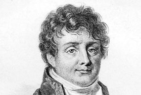
[Side-Remark: It is kind of funny to see that both super traces are the Euler characteristic. The two matrices come from completely different background which are historically pivotal: Both stories, the story of Fourier as well as the story of Leontiev are historically of extreme importance. Not only because of the fantastically groundbreaking results (Fourier theory rsp consumption-demand theory) but because of grander things even. Fourier theory was not only the start of harmonic analysis and a modern theory of partial differential equations but the birth crib of a modern view on functions. Before Fourier one has seen functions as analytic expressions only. Also the theory of Leontiev (who taught at Harvard from 1932 to 1975) not only is important for developing input-output analysis but because it was one of the first larger scale computation projects (computing on the Mark II, a relative of the Mark I at the basement of the Science center). And then, one an even larger scale, also transcending subjects, Leontiev was a proponent of quantitative science. End-Side-Remark ]

Here is a second observation which links the global sum over all matrix elements with the super sum over the diagonal:

Experimental observation: The sum over a row $\sum_y g(x,y) = (-1)^{dim(x)} g(x,x)$ .

Obviously this statement together with the super trace statement implies the global result that $\sum_{x,y} g(x,y) = \chi(G)$ . So, now it is necessary to prove this.

Update of February 19, 2017: Having noticed that the super trace of the Green function is Euler characteristic, the first reflex is to associated the diagonal entries of the Green function with curvature. This can indeed be done and the proof is quite easy if one generalizes it a bit

Here is the statement which is now a theorem (a divisor type Gauss-Bonnet theorem):

Theorem: Given a simplicial complex G, let G₁ be its Barycentric refinement. Then $\sum_x K(x) = \chi(G)$ , where the sphere curvature is defined as $K(x) = (-1)^{dim(x)} (1-\chi(S(x))$ for every vertex x in G₁.

Here is an illustration where we take a random graph and compute the sphere curvatures:

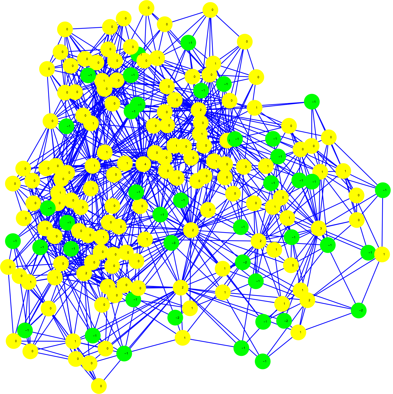
Note that the sphere curvatures are now integers, unlike in the Gauss-Bonnet-Chern story. One might not be very impressed since there is already a simple curvature on G₁, the value $\omega(x) = (-1)^{{dim}(x)}$ . But that is just the definition of Euler characteristic. /Actually, as we pointed out in the Wu story, this curvature is a Poincaré-Hopf index for the dimension functional $x \to dim(x)$ which is defined in $G_1$ and which renders the Barycentric refinement a story of hyperbolic dynamics. The sphere curvature is much more interesting. I know it is not a combinatorial invariant unlike the sphere spectrum but believe that the sphere curvature of the second Barycentric refinement is a combinatorial invariant. Sphere curvature is not an interesting curvature in the case of discrete manifolds, as it is then taking values 1 or minus 1 only depending on the dimension of the manifold and the simplex. But it becomes an interesting notion for discrete varieties and more general networks, where one gets integer values attached to points of the geometry. In other words, the sphere spectrum is a divisor!

The proof of the above statement in principle follows the same strategy as the proof of the Unimodularity theorem: rather then deforming G we deform the simplicial structure of G and see that adding a new simplex adds a value K(x). One has of course to control the total change of the curvatures near the surgery but that is no problem. In the unimodularity theory, it was a multiplication by $(1-\chi(S(x))$ .

Update of February 20, 2017: lets first recall the McKean-Singer formula for graphs: it is $str(exp(-t L)) = \chi(G)$ , where L is the block diagonal Hodge Laplacian $L=(d+d^*)^2$ and str means super trace. The formula is very transparent in the discrete as it is just a reformulation of super symmetry telling that the nonzero spectrum on the Fermionic part of odd differential forms agrees with the nonzero spectrum of the Bosonic part, the even differential forms. This symmetry implies that the super trace of $L^n$ is zero if $n$ is positive. From this the McKean-Singer formula immediately follows. This is a modern coverage of the Mc-Kean Singer formula which is in the continuum covered in the book of Cycon-Froese-Kirsch and Simon (a book which has part of my core literature as a grad student).

[Side remark:

[ A bit of personal recollections about this: as a first year graduate student at ETH, I was asked by Konrad Osterwalder to prepare for a seminar on the Patodi formula for Gauss-Bonnet. He gave me that gorgeous chapter in Cycon-Froese-Kirsch and Simon, telling me that to read that part and that the other things are less relevant. I read the chapter during a mountain retreat in Wallis and loved the super symmetry idea. The seminar eventally might have looked too ambitious for undergraduates and Osterwalder did not run that one. But the preparation work had consequences for me: I got intrigued by the almost periodic story which was told in that book. It lead me to pursue a spectral assault on the problem of positive entropy of the Standard map (today still open). Since by the Thouless formula, the Sinai metric entropy of the Standard map T(x,y) = (2x-y+k sin(x),x) is given as the von Neumann determinant of the Hessian L of the variational problem defining the dynamics (it means $\lambda=\int_{\mathbb{C}} \log|x| dk(x)$ , where dk is the integrated density of states measure defined as the functional $\phi(f) = tr(f(L))$ on the Banach space of continuous functions on the complex plane, where $tr(L) = E[ L_{xx} ]$ is the natural trace defined for operators in the cross product of $L^{\infty}(\Omega)$ and an automorphism $T$ of the probability space $\Omega$ . In this case, T is the standard map and $\Omega$ is the 2-torus equipped with the normalized Lebesgue measure. There is a natural family of Toda deformations of random Jacobi operators which has the nice feature that the average Lyapunov exponent (which initially is the Kolmogorov-Sinai entropy of T) is invariant. The naive idea was to Toda deform $L$ so that one can estimate the entropy integral, possibly in a limiting case. Such deformation ideas are of course not new. Actually, the book of Cycon-Froese-Kirsch and Simon covers in the Patodi chapter one of the most beautiful ideas in Morse theory: the Witten deformation of the Laplacian. I’m sure that I might also have been motivated by this. So, that exposure to that chapter influenced me a lot. It might also have had been part of the reason, why I had a chance for the postdoc position at Caltech. Having read that chapter also made it very easy to translate the McKean-Singer result to graph theory, where it becomes very simple as all technical parts from differential geometry and functional analysis are absent. By the way, Osterwalder is not only a pioneer in constructive quantum field theory and friend of Oscar Lanford but was also a popular teacher, covering also service calculus lectures for non-mathematicians. Some of my friends in Chemistry or Biology have had him in linear algebra and liked the lectures. I once participated in relay race on the Zürichberg, where different departments raced against each other. At that race, I had to pass the wooden relay bar to Osterwalder, who had also raced for the Math department. He is a distinguished leader in eduction, also internationally.
End Side remark.]

Now, the strange thing is that the adjacency matrix of the connection graph $G'$ of $G$ plays somehow a similar role than the Hodge Laplacian $L=(d+d^*)^2 = D^2$ , here D is the Dirac operator defined by the exterior derivative d (as defined by Betti or Poincaré). The dynamics $u(n+1)-u(n) = A u(n)$ is equivalent to $u(n-1)=(1+A)^{-1} u(n)$ which is a discrete heat flow and very much related to the heat flow exp(-t L). Formally there are relations between these two setups:

$exp(-L)=1-L+L^2/2!-\cdots, (1+A)^{-1} = 1-A+A^2- \cdots$

But the later is a divergent series. Thanks to the unimodularity theorem, we don’t have to understand this in the sense of analytic continuation but just as an elementary inverse. The McKean-Singer formula tells that the super trace of exp(-L) is the Euler characteristic. Our new Gauss-Bonnet formula tells that the super trace of $(1+A)^{(-1)}$ is the Euler characteristic too. But the reason is utterly different. It is not super symmetry. We have proven it differently and used the unimodularity theorem.

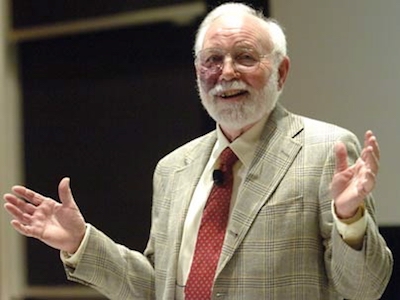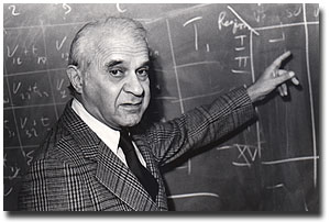
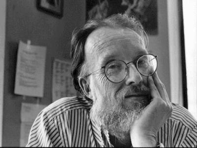
Also strange is that while the McKean-Singer deformation appears to work for any t, in the sense that $exp(-t L)$ has always a constant super trace, this does no more hold for the discrete time heat flow given by the inverse of (1+A). It is a bit strange. The analogy of a deformation is not complete, but there is no doubt that it all this is interesting quantized geometry as Green function entries are integer curvature values.


Henry McKean	Isadore Singer

Long weekend is over. Will definitely have again time for this during spring break.

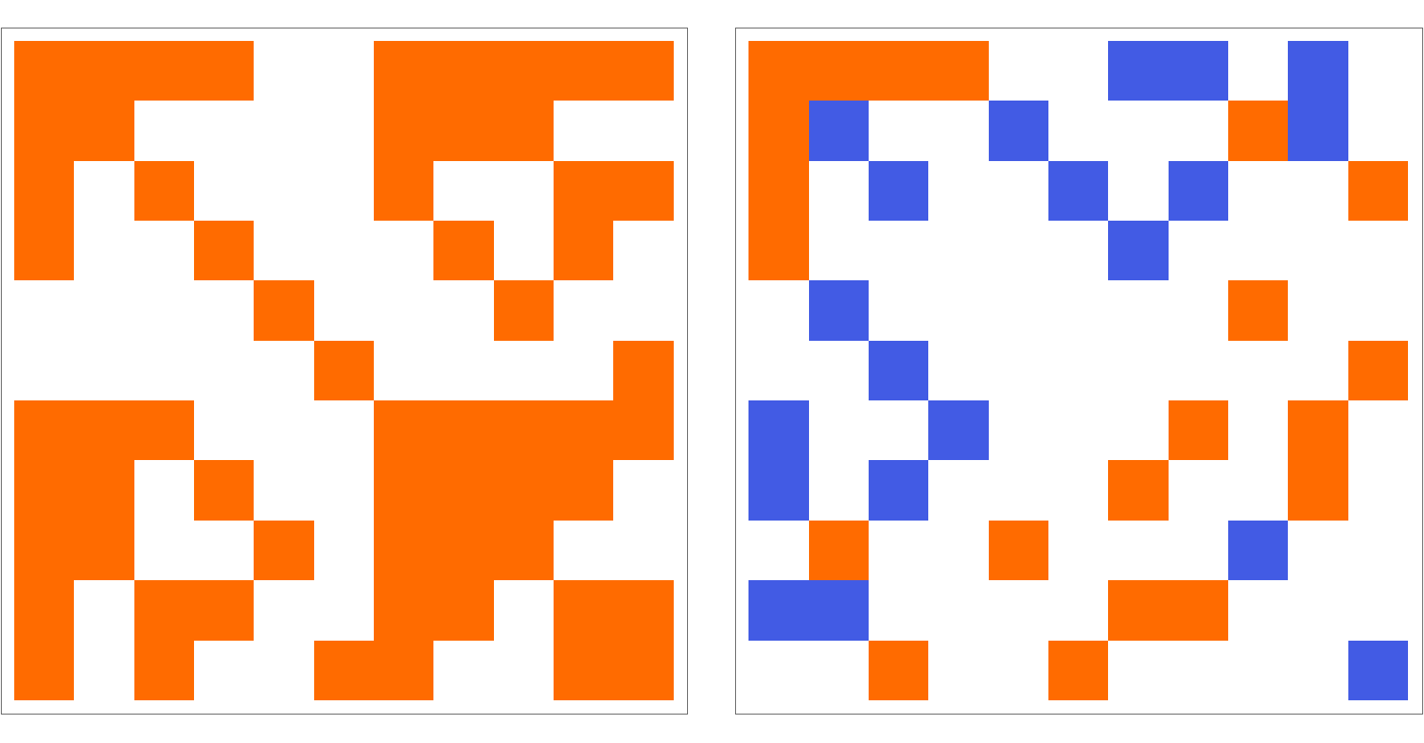
Here is a small example illustrating everything. The graph is the bunny graph. We see here the graph and its Barycentric refinement. In the refinement, the sphere curvatures are added:

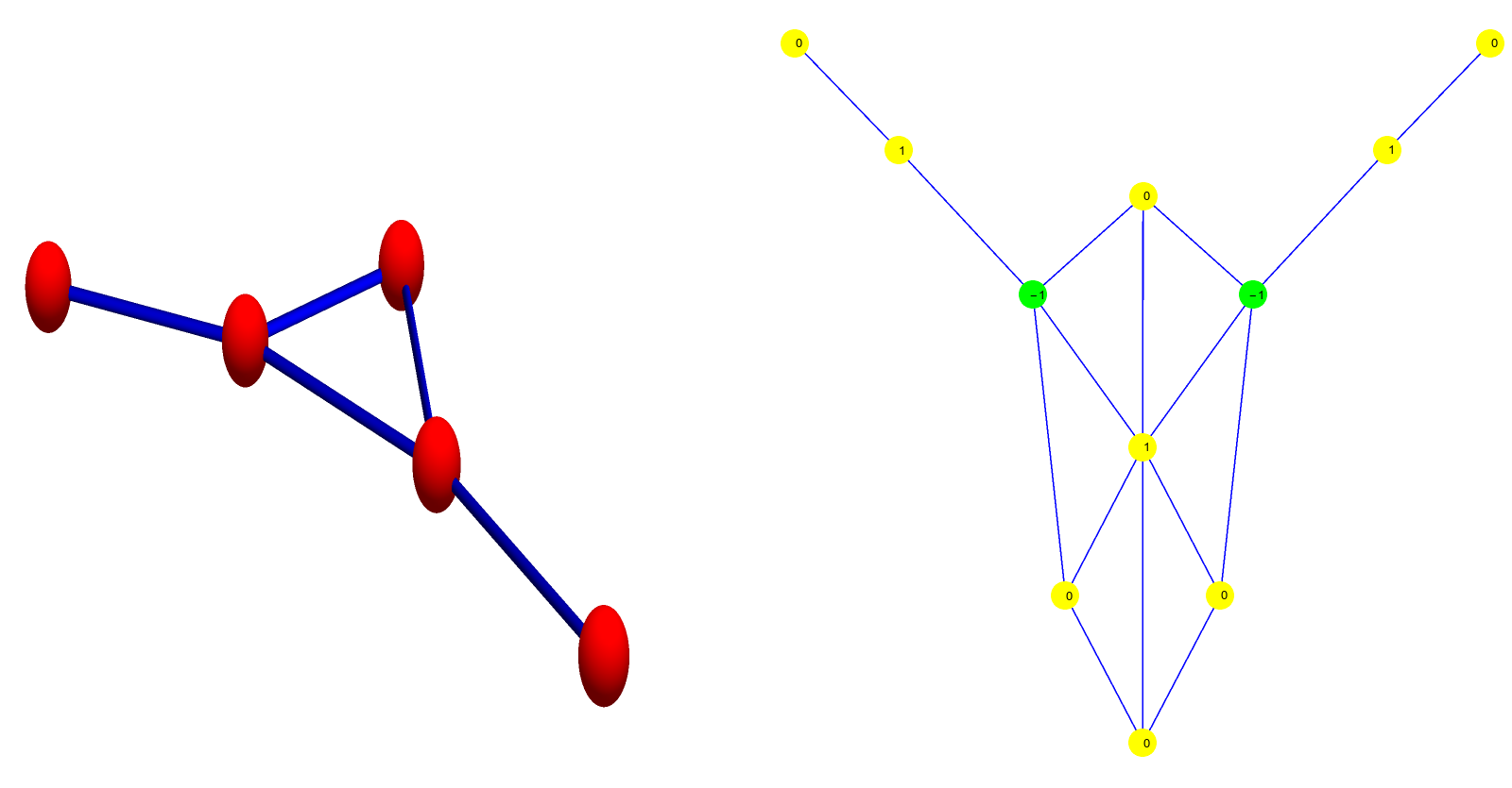
We see that the curvatures add up to 1, the Euler characteristic of G (v=5, e=5, f=1, v-e+f=X(G)). And here we see the Fredholm Connection Matrix (1+A) as well as its inverse which here only takes values 1 or minus 1. If the diagonal entries are scaled by the dimension parity factor, we get the Sphere curvature values (1, -1, -1, 0, 0, 0, 0, 0, 1, 0, 1). For every column, the sum of the Green function entries add up to the diagonal entry. The total sum over all Green function entries is 1. There are 21 entries with value 1 and 20 entries with value -1.

Here is A in ASCII graphics:

                     1   1   1   1   0   0   1   1   1   1   1

                     1   1   0   0   0   0   1   1   1   0   0

                     1   0   1   0   0   0   1   0   0   1   1

                     1   0   0   1   0   0   0   1   0   1   0

                     0   0   0   0   1   0   0   0   1   0   0

                     0   0   0   0   0   1   0   0   0   0   1

                     1   1   1   0   0   0   1   1   1   1   1

                     1   1   0   1   0   0   1   1   1   1   0

                     1   1   0   0   1   0   1   1   1   0   0

                     1   0   1   1   0   0   1   1   0   1   1

                     1   0   1   0   0   1   1   0   0   1   1

and here is its inverse in ASCII:

                     1    1    1    1    0    0    -1   -1   0    -1   0

                     1    -1   0    0    -1   0    0    0    1    -1   0

                     1    0    -1   0    0    -1   0    -1   0    0    1

                     1    0    0    0    0    0    -1   0    0    0    0

                     0    -1   0    0    0    0    0    0    1    0    0

                     0    0    -1   0    0    0    0    0    0    0    1

                     -1   0    0    -1   0    0    0    1    0    1    0

                     -1   0    -1   0    0    0    1    0    0    1    0

                     0    1    0    0    1    0    0    0    -1   0    0

                     -1   -1   0    0    0    0    1    1    0    0    0

                     0    0    1    0    0    1    0    0    0    0    -1

The main enigma at the moment is a geometric interpretation of the off diagonal entries and an explanation why the sum over each row is the sphere curvature which is the signature $\omega(x)$ of the simplex times the index $i(x)$ ). I still can not exclude that the values $g(x,y)$ are not in general some kind of Poincaré-Hopf indices. However, there are 11! = 39916800 functions on the vertices of G₁ and most likely, we would find among them a match since there are only 3¹¹ = 177147 possibilities to get rows with entries 0,1,-1. It would make more sense to see the numbers as some kind of intersection number of stable and unstable manifolds from different vertices. This makes sense since G1 has a hyperbolic dimension functional (which is a coloring) which allows to split every sphere into a stable and unstable part. I had tried a geodesic distance function but that did not work and is not expected to work also since the geodesic distance is not a Morse function.

Update of February 20: the Graph arithmetic makes the super trace formula for the Green function obvious: the super diagonal entries are nothing else than the Poincaré-Hopf values! It is just that i(S(x)) = i(S^+(x)) i(S^-(x)). Now the fact that the super trace of the identity operator is Euler characteristic is the definition of Euler characteristic and the Poincare-Hopf formula for the stable part. The new Gauss-Bonnet formula is a dual version. It is the super trace of A but can be seen as the Poincare-Hopf formula for the unstable part. Now, in a geometry with Poincare-duality, the two theorems are completely symmetric. In a variety setup with singularities or more generally for an arbitrary simplicial complex, the unstable part of a sphere can be pretty arbitrary and the Super trace becomes more interesting.

To wrap up the story about the diagonal part, we see that both McKean-Singer formulas are almost trivial when seen in the right light. The Hodge Laplacian story was due to super symmetry, the Connection Laplacian story due to a broken Poincare-Hopf symmetry, which also can be seen as a hyperbolic structure in geometry: we have stable and unstable parts at every point in the Barycentric refinement. We have already exploited that in an earlier remark: the Morse cohomology of that hyperbolic structure is not only isomorphic to the simplicial cohomology of the original graph. It is identitical. It is probably the simplest case where one can see the equivalence of simplicial and Morse cohomology. And its not something to prove but just to notice and see. Thats quite complicated in the continuum. Here it holds in full generality for all simplicial complexes!

Still, we still fight with the off diagonal parts of the connection Fredholm inverse, the off diagonal Green function values. If one looks at the vast literature and the importance of Green functions everywhere in mathematical physics (there is hardly any story which does not touch upon it), there is no doubt that there is not only an explanation, but a natural explanation. I’m currently tossing around a few possibilities but it is still an enigma.

Update of March 1, 2017: There is partial progress in identifying the off-diagonal entries. A fundamental insight is that every point in a Barycentric refinement G₁ is a hyperbolic critical point for the dimension functional dim on the vertex set of G₁: the function value dim(x) is the dimension of x when x was a simplex in G. The heteroclinic connections between different critical points produces then the Morse cohomology which is by definition the same than the original simplicial cohomology of the original complex G. As pointed out before in my “counting and cohomology paper”, it not an isomorphism but a direct identification as the exterior derivative of the Morse cohomology in G₁ is identical to the exterior derivative of the simplicial cohomology (it is the same chain complex, but that we just that we look at it from the perspective of a dynamical systems person and not from an algebraic topologists point of view. The dynamical aspect is already deeply rooted in Morse theory which is a dynamical theory for the gradient flow of a Morse function.

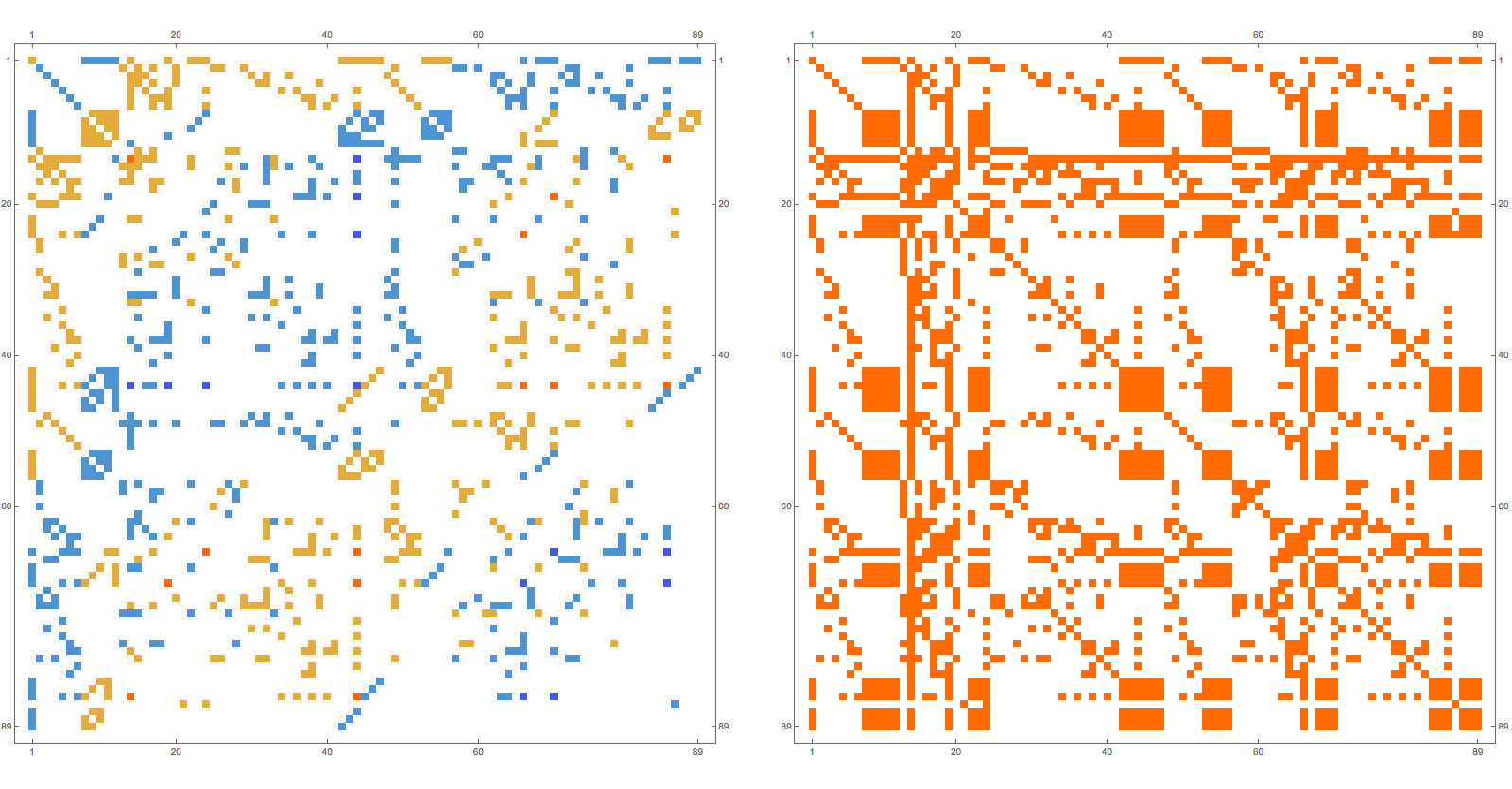
In the last few days, we looked now at the intersections of the unstable manifolds of the critical points. So, given two vertices x,y in G₁ corresponding to two faces in G, we look at the graphs W^u(x) ∩ W^u(y). The first observation is that the support of the Green function is on this intersection set. In other words, if the intersection is empty, then g(x,y)=0. We still need to prove this.

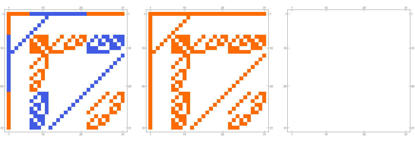
In the next picture we see first the Green function g(x,y) matrix which is the inverse of (1+A’), then we see the matrix which is 1 if the unstable connections W(x,y) = W^u(x) ∩ W^u(y) are not empty and 0 else. We see that the Green function is supported on the graphs W(x,y) of intersections.

What are the values of the intersections? We tried with Euler characteristic, Wu intersection values but not yet seriously but it seems that it only depends on x,y and the intersection W(x,y) of the unstable manifolds and not anything outside. At the moment, I would take a big bet that some kind of combination will do the trick and that it will be obvious, once seen. The Cramer formula will play a role when proving it, no doubt, but so far, it is still very opaque.

[Side remark: in an early high school, a friend of mine (Christian) and me once challenged ourselves to find a formula for the solutions of the quadratic equation. Having no resources whatsoever except TI 57 calculators for experimentation, we each looked at many cases, looked what happens if the coefficients are changed and guessed the formula, essentially by fitting with known functions. After a couple of days, we both came independently to a solution which worked. But we had no proof, just an experimental derivation. When the topic of quadratic equation was later covered in a mathematics class and we saw how easy it is with completion of squares, the experimental quest looked like a fools errant. But it shows something, we see all the time in mathematics: simple ideas, once seen, become obvious. We arrogantly then call them “trivial” and forget how hard it actually had been before seeing it. Already the Greeks solved quadratic equations geometrically by intersecting conic sections but it took more than a thousand years to go a step further and see this as a completion of square story. (And the Greeks were no fools, developed fantastic geometry and number theory, still simple ideas have escaped them) It took then a few hundred years more until algebra was developed so far that one could do this without going geometric case analysis (depending on whether the coefficients are positive or negative) as Al Khwarizmi did. Only with Vieta, one had algebraic expressions with letters representing unknowns. By the way, Christian and I raced also to get an algorithm for the Rubik cube. I needed much longer than him (several weeks more even so I was completely immersed into it, even dreaming about it). Again, once one sees an algorithm, it is obvious. Most Rubik cube solvers never went through the task to find an algorithm themselves but learn some algorithm which was already developed. (Today of course people are almost too tempted to look it up on the internet and never go through the basic fundamental research task to find the algorithm. ) That is similar than just learning the formula for the quadratic equation and then solving it. Finding an algorithm for the Rubik cube without knowledge of group theory is a bit like finding a solution of the quadratic equation without any previous insight and being agnostic about the literature. A mathematician knowing group theory can solve the Rubik cube without any resources by just applying basic principles (the Schreier algorithm for example in the theory of finitely many presented groups). But it can take a long time to find an efficient algorithm. In the case of the Rubik it can be especially challenging in the end game, here one has to develop move combinations in a relatively small stabilizer group. As a course assistant to Roman Maeder we once wrote a homework problem for the class, where with the help of a computer algebra system, the students had to write code searching the solution algorithm. It is essentially an AI task but quite dumb: the computer just looks through inductively through a narrowed down list of possibilities until the solution is found (all following Schreier-Sims). End Side remark]

From a simplicial complex G, we have looked at the heteroclinic connections between critical points. This produced the Barycentric refinement G₁ of the complex and simplicial cohomology. Then we have seen the stable connection graph between critical points. This the connection graph G’. Two points in G’ connected, if their stable and unstable manifolds intersect. Now, an other graph G` has emerged, the unstable connection graph. It connects two faces if their unstable intersections is not empty. What we saw is that the Green function adjacency matrix is zero where ever the Fredholm matrix entry of that graph is zero. We definitely have to look more closely at this graph.

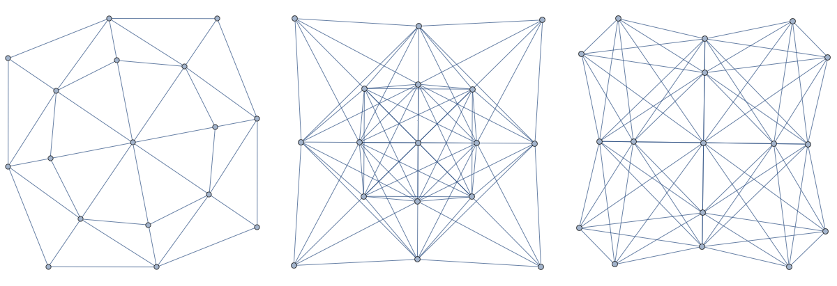
Here we see the three graphs G₁,G` and G’ for the wheel graph W₄ with 4 spikes: the Barycentric refinement G₁ is a subgraph of both G’ and G`.

Update of March 2, 2017: After some more experiments, there is some progress in the mystery of off diagonal Green function values. Let W(x,y) be the intersection of the stable manifold of x with the stable manifold of y in the Barycentric refinement G₁ of the complex G. We have seen that the support of g,
the place where g(x,y) = (1+A’)^-1_xy is non-zero, is located on the set of pairs (x,y) where W(x,y) is not empty. After correlating the cases where g(x,y) is non-zero with properties of the graph W(x,y), it appears that the Fredholm characteristic of that graph W(x,y) is a good indicator. The match seems perfect if g(x,y) is -1,0,1, but in cases, where |g(x,y)|>1, we need to know more. Also unclear is yet how we can see or interpret a larger value g(x,y) different from -1,0,1 in the graph W(x,y). (It might not even be a property of W(x,y) alone but depend on the way how the stable manifolds W(x) and W(y) intersect.)

Here is an experiment: we see first the matrix g(x,y), then the matrix which is 1, if W(x,y) is a non-empty graph with Fredholm characteristic 1, then the difference between the support of g(x,y) and that second matrix. We see that this discrepancy happens at places where the original Green matrix g is different from -1,0,1.

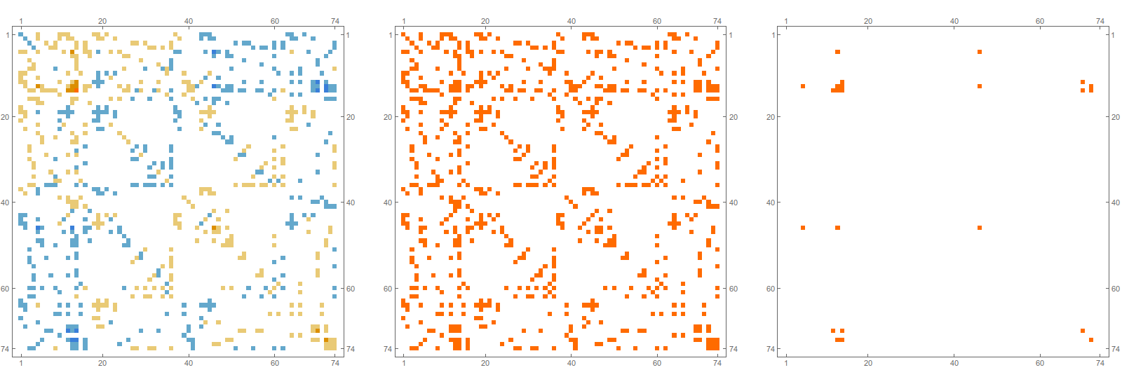
By the way, the Euler characteristic of W(x,y) is always 1. These graphs are contractible and so have not a particularly interesting topology. Since W(x,y) is contained in a collection of maximal common facets of x and y, the topology of W(x,y) is rather limited and could be classified. We need to make a list of cases and see whether we can correlate this with the integers g(x,y).

Here is a picture where G is the complete graph with 5 vertices. We see first the Green function, then the matrix which is one if W(x,y) is nonempty with Fredholm characteristic 1, then the discrepancy which is zero. But this is a case, where we have no singularities, the Green function is taking values -1,0,1 only.

The fact that for a complete graph, we have a nice picture and complete match, makes it first appear unlikely that the story in general is just local. But the hyperbolic picture is asymmetric. While the stable manifold story in a Barycentric refinement is always simple, the unstable side can be much more complicated because we can have multiple facets come together. Look at star graphs, bouquets of spheres, or windmill type graphs as appearing above, which are simplest cases, where Poincaré duality is broken in general. In a manifold setting with Poincaré duality, the picture would be already understood. For arbitrary complexes, we still have to get a grip on the Green function values. It is naturally a story of divisors but not just in a case of curves, but higher dimensional objects. If we can not get it in full generality, we would probably have to restrict to one dimensional complexes, at least to get a foot into the problem. I still hope however that it can be settled in full generality (which is often easier) and that we can match g(x,y) with some local properties of the hyperbolic connection W(x,y).

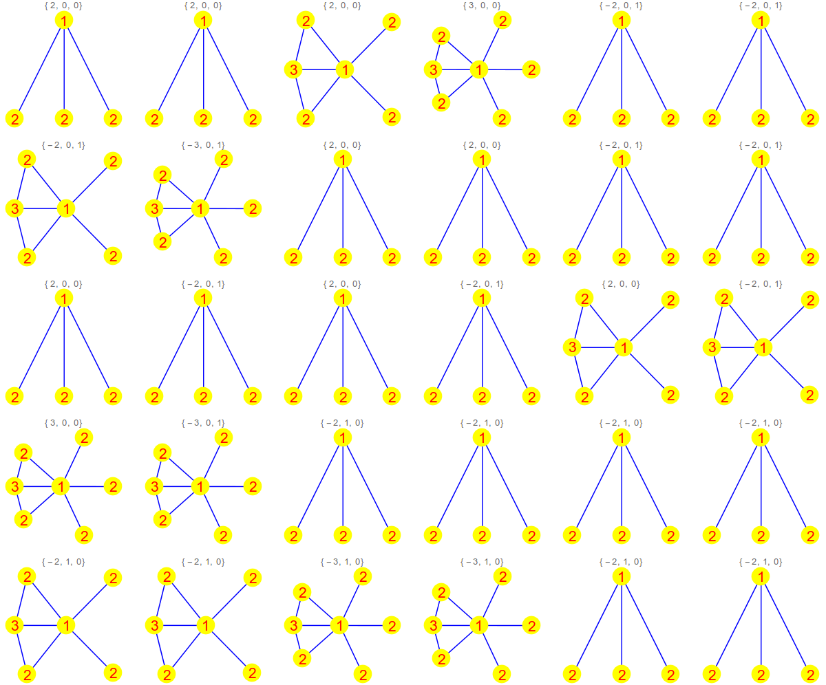
Update of March 6, 2017: after having been distracted a bit by Apollo and Artemis (Entropy and Characteristic), I still struggle to match the topology of the embedding of x,y in W(x,y) with the Green function g(x,y) value. Here are some pictures of the graphs W(x,y) for a random graph with 14 vertices. We only draw the graph if g(x,y) is different from the generic values -1,0,1 (including also the diagonal parts)

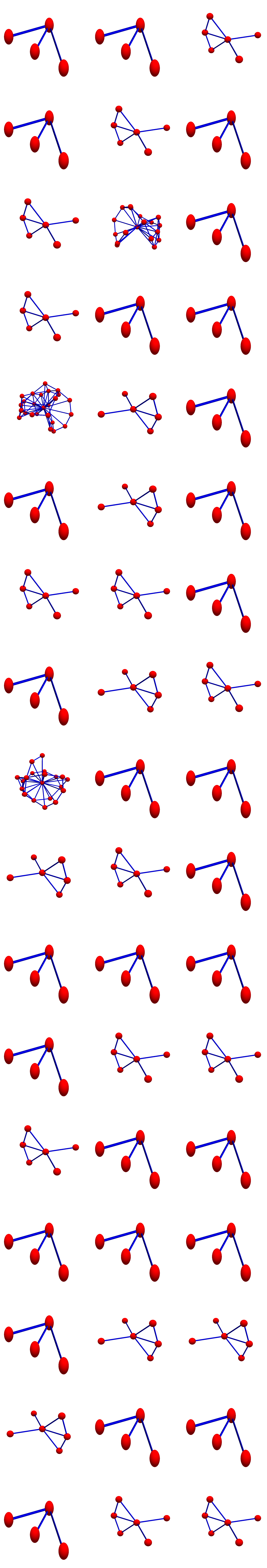
And here is a picture of the graphs W(x,y) for different x,y. We see that the graph W(x,y) alone, nor the dimension of x and y alone decides what g(x,y) is. We need also the dimension values of the individual vertices of W(x,y). In the following picture we see in each case (g(x,y),dim(x),dim(y)) in the title and then dim(z) attached to each vertex in W(x,y) (which by definition does not include x and y).

Author: oliverknill