Define the curvature K(G) of a simplicial complex as . We prove
Theorem: Given a (2d+1)-manifold G, then the expectation of the Euler characteristic of a (2d) manifold in G is 2-2K(G).
The key is the choice of probability space. Let V denote the set of vertices in G, the set of zero dimensional simplices in G and let n be its number. A configuration in defines simplicial complex that is either a (2d-1) manifold if it is not empty! I did not see the above theorem earlier because I had looked at the wrong probability space. The most obvious probability measure on is to take a Bernoulli distribution for . But what we have to take is the Bayes distribution . Bayes looked at this in a work which appeared in 1763, after his death. He proved there that this measure has the property that every event where k of the spins are 1, have probability 1/(n+1). It is somehow a very natural distribution as what happens with any Binomial distribution that taking few or large number of k has less probability. The distribution of the random variable counting the number of 1 becomes if rescaled the Gaussian distribution as the de Moivre Laplace central limit theorem shows. The Bayes distribution make this uniform. This is exactly the distribution which comes from a uniform random coloring if G is a unit sphere in a larger dimensional space. But that is exactly what renders the Poincare-Hopf indices to curvature. We have K(G) as an expectation of symmetric indices of random colorings. Now comes the index formula which I proved in 2012: we have . If S(v)=G then . So, the random manifold theorem works by just combining a few results from my “Elements of Geometry” text put together this summer. There is also a collection of shorts (1 minutes each) for each of the sections here.
There are various generalizations or versions. We can take an arbitrary finite abstract simplicial complex and get the expectation 2-X(G)-2K(G). We can also take manifolds with boundaries G for which are always manifolds with boundary. We can also take Dehn-Sommerville manifolds for which are always Dehn-Sommerville manifolds again.
The result works out numerically very well. I will post code soon. Monte Carlo runs with a few thousand manifolds already gets close to the actual value.
Also remarkable is that the expectation of Euler characteristics of sub-manifolds is a valuation. This makes sense already for manifolds with boundary. Take two balls A,B for example that intersect. Then the expectation of Euler characteristic of sub-manifolds in is known if we know it for and and .
Let us illustrate the theorem in the simplest possible case, where we look at a 1-manifold with n vertices. Submanifolds are now zero dimensional manifolds, meaning a finite collection of points. The expectation of Euler characteristic is nothing else than the number of sign changes in the sequence . While for the binomial measure the expected number of roots is n/2, for the Bayes distribution, we have the expected number of roots n/3. Therefore our theorem tells that (n/3) = 2 -2K, but that is nothing else than K=1-n/6, which is the curvature of a point in a complex which has as a unit sphere.

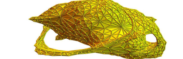


![G \to E[\chi(G_g)]](https://s0.wp.com/latex.php?latex=G+%5Cto+E%5B%5Cchi%28G_g%29%5D&bg=ffffff&fg=000000&s=0 "G \to E[\chi(G_g)]")


