Single variable Wave front Calculus

We continue to discuss an exterior derivative $d_h$ on a compact Riemannian manifold (M,g). It is a bounded operator with the property that for a k-form f, the (k+1)-form $d_hf(p)$ only depends on f located on the wave front $W_h(p)$ . It might look a bit weird at first why we want to do that but it emerged when searching for a natural multi-variable calculus in which the derivative d is bounded so that it extends to the entire Hilbert space. As explained elsewhere in more detail, we wanted originally to have fields F and geometries G on the same footing. There is a huge assymetry between these two objects. In classical calculus, we can pair a compact k-manifold G with a k-form F and form the integral $\int_G F = \langle G,F \rangle$ . For a (k+1)- manifold G and Stokes theorem is now $\langle G,dF \rangle =\langle \delta G, F \rangle$ , where $\delta G$ is the boundary. In classical geometry, there is a huge difference between geometries and fields. If we have a bounded operator however then we can extend the derivative to $L^2$ forms. Stokes theorem now becomes the almost obvious $\langle d^*G,F \rangle = \langle G,dF \rangle$ . The boundary operator is simply the adjoint of the exterior derivative.

In single variable calculus,this can be done quite easily. The discrete derivative $df(x) = [f(x+h)-f(x-h)]/(2h)$ extends to all measurable functions. If we take a geometry $G=[a,b]$ then $d^*G=([b,b+h]-[a-h,a])/(2h)$ ., the boundary of an interval is not a de Rham current located on two points but is a function again. For picdtures, see page 10 in this document from 2006/2007, written during a winter vacation in Cotuit. The 1-dimensional case is a bit misleading because one can try to generalize to higher dimension by replacing a $\mathbb{Z}$ action $T_1(x) = x+\alpha \; {\rm mod} \; 1$ with a $\mathbb{Z}^q$ action, meaning to take q commuting measure preserving transformations. This was a bit a topic in my thesis from 1993. In single variable: we can also look at the problem find the cohomology group $C^{\infty}(M)/\{f \in C^{\infty}(M), f = u(x+h)-u(x-h)\}$ , which is quite a subtle topic and central in dynamical systems theory. In the smooth case, and for Diophantine translations on M, the cohomology group is trivial. In general it is not. In the case of rational translations, it is infinite dimensional. In the traditional cohomology picture, seeing it as equivalence classes of closed forms modulo exact forms, then for irrational h, the cohomology group is uncountable, featuring a proof which Greg Hjorth had told me at Caltech. In the case of a free $\mathbb{Z}^q$ group action, the cohomology is trivial. I had worked on this a more until 2000 in this document, where the question is studied in one of the simplest set-ups: take an automorphism T of a probability space then define in the $\sigma$ algebra $\mathcal{A}$ the equivalence of events as $A \sim B$ if $A+B = C(T) + C$ where + is the symmetric difference. This defines the cohomology group of measurable sets. It is uncountable. To decide whether a given event is a coboundary $A=C(T) + C$ is hard even in the simplest cases like when A is an interval in [0,1] and T is an irrational rotation. The entire probability space $\Omega$ is a coboundary if and only if $T^2$ is not ergodic. If the probability space is finite, then the events of even cardinality are coboundaries. This analysis played a role when working on Lyapunov exponents. If you look at the Oseledec splitting of a diffeomorphism and you decide to switch from one to an other on a given set, then it very much depends on the nature of that set. If it is not a coboundary, then there will be perfect mixing between the two regions and the Lyapunov exponent will drop to zero. The decision problem whether a given cocycle has positive Lyapunov exponent or not can be difficult and is at least as hard as the cohomology problem.

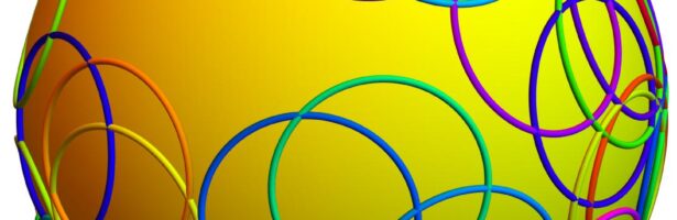
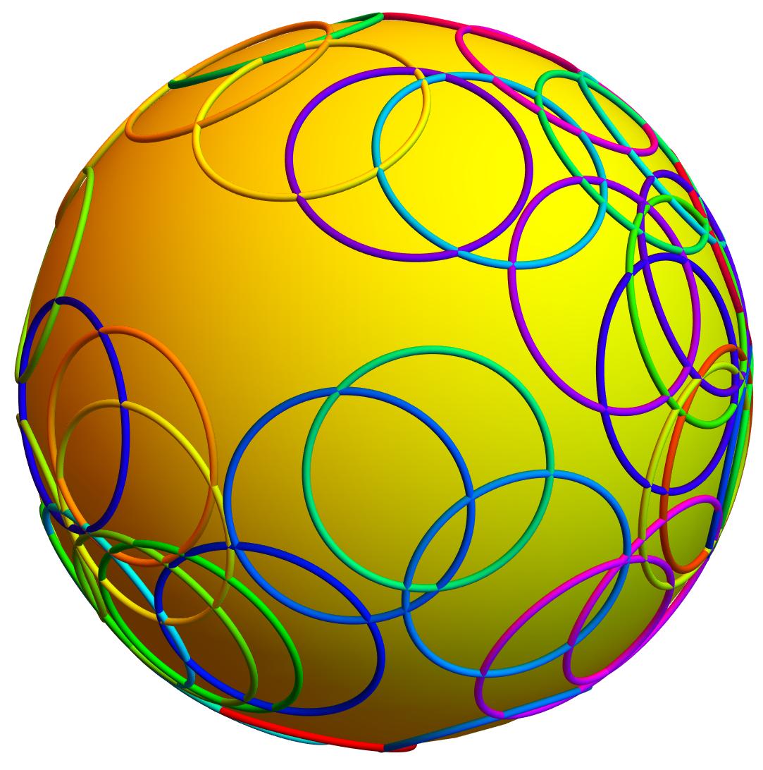
In the winter of 2010, I had started to look at the problem of building a natural quantized multi-variable calculus again and thought but now in the context of wave fronts rather than taking a discrete group action. This was certainly triggered \ by a HCRP project from 2009, a project which had started already in 2008. In the winter of 2010 and started with experiments in classical multi-variable calculus. (This had been a winter when we did not travel as we just moved to a new place in Arlington). Take a manifold like a sphere M and a vector field F, Now take at every point p the line integral along a wave front $W_h(t)$ in distance h from the point. The total curl is zero, so that one can see the line integral over the wave front as a derivative. This worked numerically and is quite easy to verify in arbitrary dimensions with arbitrary h due to cancellations. I then started to express these line integrals in terms of the Laplacian and got to the Bessel representation, suggesting $D_h = \phi(D h) D$ . Now, this winter 2025/2026, while we spent a few days in Portland, the lose ends from 2010 were picked up again and it looks now more pretty. In the following video, the one-dimensional case is discussed. There is also a bit of discussion of the zeta function of the circle and why as a scaled version of the usual zeta function it is more natural. (This was triggered by a connection between probability theory and number theory. ) I just noticed an other typo on my board of the talk. If we take $\sum_n \lambda_n^{-s}$ the Zeta function of the circle with eigenvalues $\lambda_n = n^2$ for the Laplacian we get the zeta function $\zeta_M(s) = \zeta(2s)$ , where $\zeta$ is the Riemann zeta function. The geometric zeta function is a simple variable change $s \to 2s$ but it makes some formulas more smooth as we see $s/2$ appear in the functional equation for example. The geometric xi function is now $\xi_M(s) = s(1-2s) \Gamma(s)/\pi^s \zeta_M(s)$ and satisfies the functional equation $\xi_M(1-2s) = \xi_M(2s)$ . The trivial roots of $\zeta_M(s)$ are the negative integers $-1,-2,-3, \dots$ . It is a bit a silly thought but I’m sure that if Riemann would have introduced the zeta function as a spectral zeta function, the notation $\sum_n 1/n^{2s}$ would have been entrenched. The formulas are slightly more beautiful.

Lets get back to calculus. The key point in arbitrary dimensions (I will talk about this more later) is that given a k-form f on a Riemannian manifold (M,g), we can build a (k+1) form $g=d_h f$ as follows: it is a multi-linear map skew symmetric map which assigns to (k+1) vectors $v_0,v_1, \dots, v_k$ spanning volume 1 and spanning the linear space V, the integral of f over the intersection of the geodesic sheet $\exp_p( V )$ with the wave front $\exp_p(S_h(0))$ . This is then extended in a multi-linear anti-symmetric way to all (k+1) tuples of vectors. What happens is that the value of the exterior derivative $d_h f$ only depends on the values of f on the wave front. And it does not need any smoothness of f. I hope to be able to talk about this in 2 dimensions next time. In two dimensions, one can see things still very well and also visualize why $d_h \circ d_h$ is zero.

Maybe a bit of more intuition instead which is also motivated by physics. Look at a k-form f and think about it as a field. Assume every point p in the Riemannian manifold broadcasts its value f(p) along geodesics. The rate of change $d_h f(q)$ of the field f at an other point q now only depends on the f values that can be received at time h. The derivative has become non-local but in a way that the change of f only depends on have been the f values at time h earlier.

So why looking at such a calculus?

It does not involve any limits, we do not need smoothness
All exterior derivatives are bounded, bounded operators are part of a Banach space
The calculus survives on manifolds with singularities like polyhedra.
the fields do not have to be smooth. They can be elements in the Hilbert space closure
geometric subobjects do not have to be manifolds, they again are just elements in the Hilbert space.
fields and geometries are the same (*)
isospectral Lax deformations like D’ = [B,D] work without pseudo diff operators
the boundary operation in topology is now just the adjoint of the exterior derivative.
turned around, one can see the exterior derivative as a dual to a geometric boundary operation
we involve both the language of GR (wave fronts) and the language of QM (operators on a Hilbert space)

(*) Since a few years, I used to promote such a picture end of my summer courses like in the last paragraph of this document from 2025. [PDF] and I self-quote: “Nature likes simplicity and elegance and therefore found quantum mathematics more fundamental. But a geometry in which geometries and fields are indistinguishable manifests only in the very small. ”

Author: oliverknill