The Upper bound Spectral Theorem

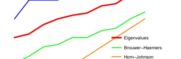
In my theorem telling that the k-th largest eigenvalue for the Kirchhoff Laplacian of a finite simple graph satisfies the bound

I use a lemma which generalizes the Andrson-Morley super symmetry result of 1985. That paper had provided a ground breaking upper bound for the spectral radius . The proof of that result is very simple if one has the idea: the Laplacian is the divergence of the gradient . In other words . From linear algebra, we know that has the same non-zero eigenvalues than . While is the 0-form Laplacian acting on functions on vertices, is the 1-form Laplacian acting on functions on edges. The entry if e,f are different edges which intersect and . The spectral radius of is of course the same than the spectral radius of and can be estimated from above by . This is the Anderson-Morley proof which is the special case of my theorem of May 2022. In order to prove the theorem, I use the Cauchy interlace theorem, induction and an upgrade of Anderson-Morley to principal sub-matrices of Kirchhoff matrices. A principal submatrix of a square matrix is obtained by deleting a few rows and corresponding columns of the matrix. I explained this upgrade either using Cauchy again or then using deformation. There is a more elegant way to see this again using super symmetry and I will make an other video on that: in a nutshell, we can extend the super symmetry result to Kirchhoff matrices of non-simple graphs with self-loops. A principal sub-matrix of a Kirchhoff matrix can always be interpreted as a Kirchhoff matrix of a non-simple graph. We still have and have a super symmetric partner for which we can estimate the spectral radius as where are the diagonal entries ordered in non-descending way. These diagonal entries can be understood as generalized vertex degrees. Every self-loop adds 1 to a diagonal. Seen in this way, the upgrade of Anderson-Morley has the same proof than the actual Anderson-Morley result from 1985. I will add this to the paper in the final version. In the youtube talk, I talked a bit about the proof which is essentially just a talk about some matrix algebra. I hope during the weekend to be able to talk about the multi-graph case.

Cauchy-Binet

The fact that and have the same non-zero eigenvalues can be seen from my generalized Cauchy-Binet formula which gives the coefficients of the characteristic polynomial of the product of of two arbitrary matrices and : (Journal version 2014 , ArXiv version 2013-2014)

(*)

Here P is a pattern, a sub-matrix indexed by finite subsets of of the same cardinality which also can be empty. The notation is a minor. In the case, where P is the empty pattern, the minor is defined to be 1. It is in general useful to declare the determinant of a matrix to be 1. This works nicely also for say partitioned matrices. Note that my determinant formula (*) above could be massaged to get the characteristic polynomial by multiplying with to get with . In the case this is equal to / In the case , this gives the Pythagorean identity which has as an application the Matrix forest theorem. An analog result deals with the pseudo determinant where depends on and . The later is just a special case, dealing with the first non-zero entry in the characteristic polynomial as this is the pseudo determinant up to a sign. Now also this has a Pythagorean aspect. If , then . In the case, where is a square matrix, then the integer is just the rank of . That Pythagorean identity immediately implies the matrix tree theorem telling that the number of rooted spanning trees in a graph is the pseudo determinant of the Kirchhoff matrix . In the case where is a matrix and the rank is maximal k=min(m,n), then the formula is the classical Cauchy-Binet result which one can find in many text books. In the case , then this is the usual determinant product formula which is always covered in any linear algebra course.

[I should add that (*) is quite a fantastic result as it is in an area of pure linear algebra, where 200 years of heavy research have been done. That no formula for the coefficients of the characteristic polynomial of a product of matrices have appeared is astounding and actually, I spent a lot of time trying to locate such a result (more time than actually finding and proving the theorem). The literature part is not an easy task as there are hundreds of linear algebra and matrix analysis books which cover Cauchy-Binet and because there are thousands of research articles on the subject. This is not just a result about a special class of matrices or some new structure which has been found in the 20th century; it is a result about a topic which is 200 years old (1812 is the date), where Cauchy and Binet independently found the first case and proved det(A B) = det(A) det(B) without having a notion of matrices yet (!) and which is under heavy investigation since, due to the vast amount of applicability of determinants and matrices in sciences. I myself got exposed to the history of Cauchy-Binet by a conversation with Shlomo Sternberg from 2007 and have tried to track down things a bit in 2009. Shlomo had been interested to locate the exact time when matrix multiplication first appeared. It was definitely past the introduction of determinants which origins from the 17th century (Seki and Leibniz independently). But matrix analysis only appeared in the 18th century. There is an article of Knobloch from 2013 which illuminates a bit the history. Leibniz has worked in particular in the case up to n=4 and saw recursive notions or properties like that that interchanging rows or columns changes the sign.]

In the case , which was a case I had been particularly interested, one gets a Fredholm determinant and Fredholm determinants are especially dear to me as they behave nicely in infinite limits, because they lead to connection matrices which are unimodular. (By the way, Sajal Mukherjee and Sudip Bera have found an other, more elegant proof of the unimodularity theorem in 2018.) The formula (*) immediately implies that we can replace F and G with its transpose. While and almost trivially have the same eigenvalues as they are transposes of each other. The matrices and have different size and the fact that their non-zero eigenvalues agree is less trivial. Percy Deift wrote in 1978 an entire paper devoted to the applicability of this commutation formula. The formula appears for example in the theory of integrable systems (a topic I worked in my PhD thesis too, in particular with Toda systems which are discrete versions of KdV systems.). In quantum mechanics knows how to compute the spectrum of the quantum harmonic oscillator: if and are the creation and annihilation operators, (where $\latex D f (x) = f'(x)$ is the differential operator giving the derivative related to the momentum operator P=-iD and Xf=xf is the position operator), then the Hamiltonian of the quantum harmonic oscillator can be written as , the commutation formula for the quantum harmonic oscillator. Since and have the same non-zero eigenvalues, we can from the commutation formula see that the eigenvalues are , where n is a non-negative integer. Given the ground state one can get the other eigenfunctions by bootstrapping using the creation operator. The relation is a version of the canonical commuation relation like between momentum P and position Q. Note however that in our case where we deal with incidence matrices F of graphs, the matrices F are not square matrices if the number of vertices and edges are not the same. Still there is a quantum field aspect of calculus if one uses the matrix which acts on all differential forms (all functions on simplices). Now and $(d^*)^2=0$ like for annihilation and creation operators. The operator is the Dirac matrix which in the graph case again is a matrix where is the number of complete subgraphs. Now is the Hodge Laplacian, which is block diagonal and which contains the form Laplacians as blocks. The first block is the Kirchhoff matrix ! McKean-Singer noticed a symmetry: the non-zero eigenvalues of the even forms are the non-zero eigenvalues of the odd forms. If one looks at the skeleton complex of a graph which only consists of vertices and edges (a castration of graphs which unfortunately has been performed in most textbooks of graph theory in the 20th century who consider graphs to be one-dimensional simplicial complexes. There is so much more to them!), then there the 0-form Laplacian and the 1-form Laplacian have the same non-zero eigenvalues. This is well known in linear algebra. The matrices and always have the same non-zero eigenvalues. In the Laplacian case and is the 1-form Laplacian. In the Kirchhoff case, the operation which K performs is first mapping a 0-form into a 1-form and then pushing it back to be a 0-form. In the 1-form case, a 1-form is first pushed to be a 0-form and then back to be a 1-form. In general, if the lobotomy on graphs has not been done and the full Whitney complex has been taken, then the Laplacian on 1-forms is since we have now two possibilities: we can apply the annihilation operator first to get to a 0-form then apply the creation operator to get a 1-form again. Or then, we can apply the creation operator to get a 2-form and then apply the annihilation operator to get back a 1-form.

McKean-Singer

The fact that the non-zero eigenvalues of the 0-form Laplacian and the 1-form Laplacian are the same is a special case of McKean-Singer super symmetry. I talked about this a lot in this blog or youtube videos too but there is a completely analog Hodge theory in the graph case than in the continuum. Define differential forms as functions on simplices and define exsterior derivatives as Poincare or Betti did but write this exterior derivative d as a matrix if N is the number of simplices (=complete subgraphs = cliques) in the graph. Now is the Dirac operator of the graph. [ By the way, it is a bit vexing why the founders of algebraic topology have only looked at the individual incidence matrices and not the full matrix . If yes, Hodge theory could have been invented much earlier. Atiyah showed how explosive the mix of Hodge theory and Dirac theory can become. He has mused once in a talk how lucky he was that Hodge and Dirac who were office neighbors in the same department but rarely talked to each other, allowing him to take these explosive ingredients and combine them to explosions like the Atiyah-Singer index theorem.] Now is the Hodge Laplacian. This is a block diagonal matrix. If are the blocks, then the nullity of is the k’th Betti number. The kernel of , the space of harmonic k-forms is the k-th cohomology group of the graph. Of course, if G has as a geometric realization a smooth manifold, then these is the cohomology of the manifold. The McKean-Singer supersymmetry result deals with the operator and . Let denote the set of non-zero eigenvalues of a matrix . This is the non-zero spectrum. The McKean-Singer super symmetry assures

This implies for all $m$, where is the super trace. The Euler characteristic of the graph is . The McKean-Singer formula is now

The above mentioned fact that the non-zero eigenvalues of and agree is the McKean-Singer super symmetry in the case when dealing only with a simplicial complexes which are one-dimensional.