Energy Entropy competition
We have seen some structural similarities between Euler characteristic and entropy. These two functionals share similar uniqueness features, behave nicely with respect to renormalization maps and both feature central limit theorems. They also be considered together. Due to the boundedness of the Green function, classical Newtonian potential theory and thermodynamic notions can be considered on simplicial complexes without any technical difficulties. Especially the Laplacian L=1+A’ with the Newtonian potential  = g(x,y)=L^{-1}") on a graph. (Any geometry with Laplacian L produces Green functions g(x,y) and so Newtonian potentials. The prototype is the Laplacian
on a graph. (Any geometry with Laplacian L produces Green functions g(x,y) and so Newtonian potentials. The prototype is the Laplacian  , where the potential is the Newton potential Vx(y)=1/|x-y|). In our case, the potential is remarkably finite. The entries are even integers, which is even more remarkable. If we add the interaction energy given by the geometry to entropy, there is a competition between two functionals: the interaction energy U wants the probability measures to clump together, while entropy S likes the measures to spread out. This interesting interplay allows richer phenomena and in the case of classical thermodynamics, enables conditions away from chaos and static energy sinks, conditions in which life possible. With entropy alone, nature would be chaos, with energy alone, the world would be at some frozen minimum. Entropy shakes things up, energy organizes. The insight for this has been known since a long time. In chemistry, it is one of the most basic principles. In statistical mechanics models it is known under the name Peierls argument. In a mathematical context, the principle was probably first formulated by Gibbs. Indeed, one of the most important equilibria, the Gibbs distribution is such a minimum. A nice booklet of Rufus Bowen features this example in the introduction. It is important as it explains why the configuration probability in statistical mechanical models is the Gibbs distribution. I always use this Lagrange problem in multivariable calculus classes example: the free energy
 ") is minimized by the Gibbs distribution
is minimized by the Gibbs distribution /\sum_j e^{-E_j}") . (More generally, if U-S is replaced by U-TS with some temperature parameter T=1/β then
. (More generally, if U-S is replaced by U-TS with some temperature parameter T=1/β then /\sum_j e^{-\beta E_j}") .) This prototype problem shows how more interesting measures can emerge if energy minimization and entropy maximization competes. In geometry, the principle could select interesting geometries and probability distributions (in the form of wave function amplitude squares
.) This prototype problem shows how more interesting measures can emerge if energy minimization and entropy maximization competes. In geometry, the principle could select interesting geometries and probability distributions (in the form of wave function amplitude squares  ). It is the basic problem to understand “space” “time and “matter” to quote a book title of Herman Weyl. But now, we are in a setup, where the problem of space and matter combined can be studied even for very small geometries and which it is pure mathematics. It is not combinatorics alone if one allows the wave to take values in the continuum like the complex numbers or quaternions, but a purist could remedy this by discretization of the target space and look at integer valued waves and also get closer to the “particles and primes” story. Anyway, the set-up is a situation, where one can study waves and geometries together in a single variational problem. I’m actually not aware that such finite geometric variational problems mixing geometry and fields have been studied. (but statistical mechanics is such a large field that it well might have been). Even extremizing Euler characteristic alone appears not studied much, maybe because due to the discrete values of the functional, classical calculus of variation methods do not apply. Some experiments with variational problems on graphs can be seen here.
|
|
|
|
| Gibbs |
Heisenberg |
Ising |
Lenz
|
Basic functionals in statistical mechanics
It is custom in statistical mechanics to add more quantities like a multiple of the volume V to energy and entropy. Now, with enthalpy U+p V with a pressure parameter p. The functional to consider now is the free energy F = U + p V – T S, where T is a temperature parameter. In our case, U is the Euler characteristic, as we have seen that the sum over all energy values is Euler characteristic. We will say more about energy U later on as this is the current focus. One could to to add even more functionals, like an interaction term in the form of Wu characteristic  = \sum_{x \sim y} \omega(x) \omega(y)") , where the sum is taken over all interacting simplices and
, where the sum is taken over all interacting simplices and  = (-1)^{dim(x)}") is the Wu characteristic of a simplex. Related to that one can look at some Lie group valued field, the wave function and mix it into the bag. Examples are
is the Wu characteristic of a simplex. Related to that one can look at some Lie group valued field, the wave function and mix it into the bag. Examples are , SU(2)") valued fields (meaning that the sphere is 0,1 or 3 dimensional, the reason for these groups that they are the only spheres in Euclidean space which are also groups). We have then the Heisenberg action
valued fields (meaning that the sphere is 0,1 or 3 dimensional, the reason for these groups that they are the only spheres in Euclidean space which are also groups). We have then the Heisenberg action  = \sum_{x \sim y} \psi(x) \cdot \psi(y)") which is in the zero-dimensional case the Ising-Lenz action
which is in the zero-dimensional case the Ising-Lenz action  = \sum_{x \sim y} \sigma(x) \sigma(y)") . By the way, in the mathematical physics community there is some satisfaction to the maybe unjust nomenclature “Ising model” as Ising got the problem from Lenz, but carries Ising’s name even in two dimensions, which has not been tackled successfully by Ising. The revenge is the uncertainty of the spelling of Ising as there is an obvious phase transition between the English and German spelling. (It is a small satisfaction indeed, but nevertheless sweet). Also, according to mathematical physics community rumors (spread maybe to balance a bit the maybe unjust luck of Ising, hitting the jackpot), Ernst Ising (1900-1998) spent the later part of his life collecting literature mentioning the Ising model. As the Wikipedia entry mentions, every year about 800 papers appear related to that model. This perfectly explains why Ising was unable to do much new physics later: keeping track of his own legacy had become a demanding full time job.
. By the way, in the mathematical physics community there is some satisfaction to the maybe unjust nomenclature “Ising model” as Ising got the problem from Lenz, but carries Ising’s name even in two dimensions, which has not been tackled successfully by Ising. The revenge is the uncertainty of the spelling of Ising as there is an obvious phase transition between the English and German spelling. (It is a small satisfaction indeed, but nevertheless sweet). Also, according to mathematical physics community rumors (spread maybe to balance a bit the maybe unjust luck of Ising, hitting the jackpot), Ernst Ising (1900-1998) spent the later part of his life collecting literature mentioning the Ising model. As the Wikipedia entry mentions, every year about 800 papers appear related to that model. This perfectly explains why Ising was unable to do much new physics later: keeping track of his own legacy had become a demanding full time job.
Why look at functionals?
The reason is at the core of all successful physics: maxima and minima appearing in the calculus of variations are always interesting. Paths in a Hamiltonian system are after a Legendre transform solutions of a variational principle. Field theories are Lagrangian based. The solutions to the Einstein equations are extrema of the Hilbert action (Hilbert got this just about at the same time than Einstein got the field equations. GR as almost a mathematicians discovery, similarly as special relativity had been seen already by Poincaré, who was so mad on Einstein that he never quoted him. To be fair to Einstein, Poincaré hardly saw the ramifications and importance of the Lorentz symmetry in physics but saw it just as a good symmetry. It is an interesting story.). Also the standard model in particle physics is an extremely successful theory and based on some Lagrangian incorporating various fields. The universality idea allows often to get rid of free parameters but the mathematics can be formidable even in very simple setups. It also explains some other phenomena like symmetry breaking which happens if multiple minima can coexist or phase transitions which are bifurcation parameters of the critical points. In the graph or simplicial complex setup, the infinite volume limit is done in the form of Barycentric limits. It is different than infinite lattice limits or renormalisation schemes because under Barycentric refinements, the vertex degree grows exponentially.
A concrete example coupled to a wave
In our case, with a finite simplicial complex in which Euler characteristic is a natural “internal energy”, it is promising for example to look at the functional  = \chi(G) - p H(\psi) + T S(|\psi|^2)") with a wave functions with
with a wave functions with  . Now
. Now ") takes care of the internal energy of the geometry, the Heisenberg action
takes care of the internal energy of the geometry, the Heisenberg action ") takes care of the energy of the field. The amplitude square leads then to a probability measure on the geometry and S is its entropy. Taking
takes care of the energy of the field. The amplitude square leads then to a probability measure on the geometry and S is its entropy. Taking  + T S(|\psi|^2") without the Euler characteristic is the classical Ising or Heisenberg model as the extrema lead to the Gibbs measures which then in these models are considered in a limit.
without the Euler characteristic is the classical Ising or Heisenberg model as the extrema lead to the Gibbs measures which then in these models are considered in a limit.
[Added March 11 2017: By the way, the Gibbs measures in the infinite limit are also known under the name DLR measure named after Dobrushin, Lanford and Ruelle. I’m fortunate that I could take classes from all three at ETH. Both Dobrushin and Ruelle gave semester long post graduate lectures, Dobrushin on classical statistical mechanics and Ruelle on Zeta functions. Its maybe not an accident relations with these characters appear: 1/det(1+A’) is a special value of a Bowen-Lanford zeta function which has been generalized vastly by Ruelle. Lanford was also very interested in finite notions of dynamical systems, in particular in the context of (still poorly understood) effects when a finite computer simulates a continuum dynamical system. In the hyperbolic case (hyperbolicity appears for simplicial complexes naturally in the Barycentric refinement, as the gradient flow of the dimension functional is hyperbolic leading to interesting structure), there is more hope to understand the discrete-continuum limit, notably due to the shadowing lemma. The problem is that one often has only weak type of hyperbolicity or that one is unable to prove it.
]
When changing the complex G, then the size of the matrices representing the Laplacians changes considerably and change the variational problem setup for the probability measure p. A minimum is a configuration for which any modification of the complex (adding a new face or removing a face) makes ") larger or keeps it the same and where any change of the wave
larger or keeps it the same and where any change of the wave  does the same. Now if we have such a configuration, we both have fixed the geometry as well as the initial condition for a wave evolution. The parameters p and T are tuned to be critical in the sense that the functional is not smooth there in the Barycentric limit. Now we have a physical toy model which could be compared with real physics. As pointed out here, the case of quaternion values is also promising. The restriction onto the unit sphere of
 ") produces then a probability measure for which the entropy is taken.
produces then a probability measure for which the entropy is taken.
Wu characteristic variation
In order to experiment, one would have to remain open minded and possibly allow to modify the functionals. It could make sense for example to replace the Euler characteristic with Wu characteristic or then combine various Wu characteristics together similarly as adding higher order terms to field theories. There are some mathematical connections between the functionals. The Wu characteristic is a generalized super trace  = {\rm tr}( (1+A') J)") , where J is the checkerboard matrix
, where J is the checkerboard matrix ^{dim(i)+dim(j)}") . The relation is that
. The relation is that ") is the Fredholm characteristic and that
is the Fredholm characteristic and that ^{-1}") leads to the Euler characteristic in the form of
leads to the Euler characteristic in the form of ^{-1} I) = \chi(G)") , where
, where  . So, both functionals, Euler characteristic
  (total internal energy) and Wu characteristic
  (total interaction energy) are spectral notions. By the way, the Wu characteristics
 ") all share similar properties like the Euler characteristic. Each has its cohomology and a corresponding Euler-Poincaré formula expressing the characteristic as a super sum over Betti numbers. Interaction cohomology can give more information about a complex than simplicial cohomology. It can distinguish spaces like the Möbius strip and the cylinder which are homotopic so that their difference can not be detected by simplicial cohomology.
all share similar properties like the Euler characteristic. Each has its cohomology and a corresponding Euler-Poincaré formula expressing the characteristic as a super sum over Betti numbers. Interaction cohomology can give more information about a complex than simplicial cohomology. It can distinguish spaces like the Möbius strip and the cylinder which are homotopic so that their difference can not be detected by simplicial cohomology.
The variational problem
For every p and T we can look for minimizing measures of the free energy  - p V(G) - T S(p)") , where V could be volume (number of facets in the complex G) or some interaction correlation energy
, where V could be volume (number of facets in the complex G) or some interaction correlation energy  \cdot \psi(y)") and where S is the entropy of the probability measure
and where S is the entropy of the probability measure =|\psi(x)|^2") . This is a finite dimensional variational problem and can be treated with calculus as long as is nowhere 0. However, this is not the only thing which can vary. We can also modify the graph G which is a discrete variational problem not accessible through classical calculus. We hope that except at some few exceptional points, the functional F(p,T) selects some interesting geometry G and remains smooth (as a function of p an T) in the Barycentric limit at most places leaving some interesting critical points to consider. When picking the critical parameters (p,T) we should then get to a minimum, which could lead to interesting graphs. This is the classical story of thermodynamics. (It can hardly be more classical than that.) What happens in those setups is that the initially free parameters like pressure p and temperature T can get fixed through the requirement to be critical. In that case, some universal new constants appear near the critical points. Universal means that these constant do not depend on anything. The wave function of course then can be the initial condition for a wave evolution (which is always fundamentally equivalent to the Schroedinger equation for the Dirac operator on the simplicial complex) and which emerges naturally by letting the exterior derivative evolve in the isospectral set. While the mathematical difficulties for finding the extrema could be formidable, the importance could be that one can experimentally study small physical worlds, selected by variational principles. Find the minimum on a graph with very few vertices can be done with the help of a computer. By just taking internal energy alone, I have seen experimentally that (Zykov) non-prime graphs like complete bipartite graphs often became minima. Together with waves, this could become more interesting to study as one can also watch also the probability distributions.
. This is a finite dimensional variational problem and can be treated with calculus as long as is nowhere 0. However, this is not the only thing which can vary. We can also modify the graph G which is a discrete variational problem not accessible through classical calculus. We hope that except at some few exceptional points, the functional F(p,T) selects some interesting geometry G and remains smooth (as a function of p an T) in the Barycentric limit at most places leaving some interesting critical points to consider. When picking the critical parameters (p,T) we should then get to a minimum, which could lead to interesting graphs. This is the classical story of thermodynamics. (It can hardly be more classical than that.) What happens in those setups is that the initially free parameters like pressure p and temperature T can get fixed through the requirement to be critical. In that case, some universal new constants appear near the critical points. Universal means that these constant do not depend on anything. The wave function of course then can be the initial condition for a wave evolution (which is always fundamentally equivalent to the Schroedinger equation for the Dirac operator on the simplicial complex) and which emerges naturally by letting the exterior derivative evolve in the isospectral set. While the mathematical difficulties for finding the extrema could be formidable, the importance could be that one can experimentally study small physical worlds, selected by variational principles. Find the minimum on a graph with very few vertices can be done with the help of a computer. By just taking internal energy alone, I have seen experimentally that (Zykov) non-prime graphs like complete bipartite graphs often became minima. Together with waves, this could become more interesting to study as one can also watch also the probability distributions.
Internal energy of a geometry
There is a general way to get internal energy from geometry: given a finite geometry G with some sort of Laplacian L on a Hilbert space H, one has a potential in the form of a Newtonian potential. Examples of Laplacians are the adjacency matrix, the Hodge Laplacians ^2") on k-forms or the Fredholm matrix 1+A, where A is the adjacency matrix. Given a Laplacian, the Green functions are defined if a basis for the Hilbert space H, we can look at the matrix entries
on k-forms or the Fredholm matrix 1+A, where A is the adjacency matrix. Given a Laplacian, the Green functions are defined if a basis for the Hilbert space H, we can look at the matrix entries  = L^{-1}_{x,y}") which might be unbounded. We write
which might be unbounded. We write ") and call this the potential of y at the point x. Thinking in physics terms, we can interpret this as the potential energy between x and y. It is the classical gravity defined by the geometry. Classically, the potential is the Newtonian kernel. The fact that the total interaction energy is the Euler characteristic is interesting, as there is also an other interpretation as a discrete version of a Hilbert action. The Hilbert action is now identical to the internal energy. To see the classical mathematical approaches to gravity ( Gauss law for classical mechanics) and general relativity (Hilbert’s derivation of general relativity) identified is encouraging. In the continuum a connection between the Gauss and Hilbert functionals is obtained in the limit where the speed of light goes to infinity and the metric tensor is expanded about the flat metric).
and call this the potential of y at the point x. Thinking in physics terms, we can interpret this as the potential energy between x and y. It is the classical gravity defined by the geometry. Classically, the potential is the Newtonian kernel. The fact that the total interaction energy is the Euler characteristic is interesting, as there is also an other interpretation as a discrete version of a Hilbert action. The Hilbert action is now identical to the internal energy. To see the classical mathematical approaches to gravity ( Gauss law for classical mechanics) and general relativity (Hilbert’s derivation of general relativity) identified is encouraging. In the continuum a connection between the Gauss and Hilbert functionals is obtained in the limit where the speed of light goes to infinity and the metric tensor is expanded about the flat metric).
Classical capacity
Newtonian potentials naturally lead to notions of capacity. The most prominent one is capacity in the complex plane, where it is called logarithmic capacity. It is relevant in spectral questions or then in the theory of complex dynamics. As usual when dealing with Newton potentials in Euclidean space, one has to overcome difficulties due to singularities. The potential theoretical energy of a measure  in the complex plane is
  d\mu(w)") where there is a problem at the diagonal where z=w. But things work nicely for many sets and the minima are nice measures giving a finite internal energy. There is a notion of “polar sets” which are exactly the sets for which the energy has no finite minimum. Part of my theses dealt with operators which have the spectrum on Julia sets. Julia sets have natural measures, equilibrium measures and these are then just the density of states of the operators. In some sense, that story is a quantisation of Julia sets as it inverts the map T(z)=z2 + c on operators leading (as in the complex plane) to an attractor which happens to be the hull of an almost periodic operator. The limiting dynamics jumping between adjacent nodes in the limiting space is the naturally the addition in the dyadic group of integers (one of the most beautiful spaces as it is a compact Abelian group with a smallest unit). In some sense, the dyadic group of integers takes the best properties of the circle and the integers. This group can also be seen as a von-Neumann-Kakutani renormalisation limit of dynamical system (under 2:1 integral extension operation) as shown in my thesis or can be seen as the limiting case of the Barycentric renormalization map in the one dimensional case. In dimensions 2 and larger, we have no clue yet what the limiting space is. For more, see the Universality in Barycentric refinement story.
where there is a problem at the diagonal where z=w. But things work nicely for many sets and the minima are nice measures giving a finite internal energy. There is a notion of “polar sets” which are exactly the sets for which the energy has no finite minimum. Part of my theses dealt with operators which have the spectrum on Julia sets. Julia sets have natural measures, equilibrium measures and these are then just the density of states of the operators. In some sense, that story is a quantisation of Julia sets as it inverts the map T(z)=z2 + c on operators leading (as in the complex plane) to an attractor which happens to be the hull of an almost periodic operator. The limiting dynamics jumping between adjacent nodes in the limiting space is the naturally the addition in the dyadic group of integers (one of the most beautiful spaces as it is a compact Abelian group with a smallest unit). In some sense, the dyadic group of integers takes the best properties of the circle and the integers. This group can also be seen as a von-Neumann-Kakutani renormalisation limit of dynamical system (under 2:1 integral extension operation) as shown in my thesis or can be seen as the limiting case of the Barycentric renormalization map in the one dimensional case. In dimensions 2 and larger, we have no clue yet what the limiting space is. For more, see the Universality in Barycentric refinement story.
[Side remark added March 10, 2017: having tried (following Herman and others) for over a decade to use potential theoretical methods for proving a problem in ergodic theory, I have a love-hate relationship with potential theory. Love because potential theory worked well to show that positive Lyapunov exponent is dense in SL(2,R) cocycles; then pain because of failures. In the first weeks of being a grad student, I constructed the analytic map  = (z w e^{z-u},w e^{z-u},u v e^{u-z}, v e^{u-z})") which has the property that it preserves the invariant the tori
which has the property that it preserves the invariant the tori  and induces there simultaneously all the Chirikov Standard maps
  = (x+y+ c \sin(x), y+ c \sin(x))") . The idea had been that because of pluri-subharmonicity of the Lyapunov exponent, one can estimate the Kolmogorov-Sinai entropy of
. The idea had been that because of pluri-subharmonicity of the Lyapunov exponent, one can estimate the Kolmogorov-Sinai entropy of  from below by
 ") . This bound matches the experiments and is rigorous (due to Herman) if the same cocycle is assumed to fiber over an irrational rotation. I showed this “proof” to Moser who over-night saw the problem: the torus S is not the boundary of a polydisc so that the pluri-subharmonic argument does not apply. [Moser of course is known best for KAM and integrable models like Calogero-Moser but also a specialist in higher dimensional complex analysis which I myself learned in a seminar of his, where the topic had been a beautiful multidimensional stability theorem in several complex variables.] I tried for a few years to mend this but without success. When the approach of combining potential and Schroedinger and multi linear methods failed and time for my fellowship in Texas ended, I made a last desperate attempt with a completely new approach: the paper on fluctuation bounds makes (a minor but still some) progress in a very classical area of complex analysis by introducing a method of homogenisation, allowing to bound lower fluctuations A of a subharmonic function on a circle from upper fluctuations B on that circle. In some sense it supplements the Harnack inequality for the harmonic part of a subharmonic function, where lower and upper fluctuations are comparable. The Harnack inequality gives a trivial inequality A ≤ B. For potentials this is of course false but the right hand side can be replaced by an infinite sum which often can be estimated. It allows to make some subtle statements about continuity of subharmonic functions depending on the continuity properties of its Riesz measure. End side Remark.]
. This bound matches the experiments and is rigorous (due to Herman) if the same cocycle is assumed to fiber over an irrational rotation. I showed this “proof” to Moser who over-night saw the problem: the torus S is not the boundary of a polydisc so that the pluri-subharmonic argument does not apply. [Moser of course is known best for KAM and integrable models like Calogero-Moser but also a specialist in higher dimensional complex analysis which I myself learned in a seminar of his, where the topic had been a beautiful multidimensional stability theorem in several complex variables.] I tried for a few years to mend this but without success. When the approach of combining potential and Schroedinger and multi linear methods failed and time for my fellowship in Texas ended, I made a last desperate attempt with a completely new approach: the paper on fluctuation bounds makes (a minor but still some) progress in a very classical area of complex analysis by introducing a method of homogenisation, allowing to bound lower fluctuations A of a subharmonic function on a circle from upper fluctuations B on that circle. In some sense it supplements the Harnack inequality for the harmonic part of a subharmonic function, where lower and upper fluctuations are comparable. The Harnack inequality gives a trivial inequality A ≤ B. For potentials this is of course false but the right hand side can be replaced by an infinite sum which often can be estimated. It allows to make some subtle statements about continuity of subharmonic functions depending on the continuity properties of its Riesz measure. End side Remark.]
Capacity of a network
But potential theory works well on a network if we take the Laplacian L=1+A’, where the potential is finite. Given a probability measure on a graph, we can define  = exp(-U(\mu))") , where
, where  = \sum_{x,y} \mu(x) \mu(y) g(x,y)") is a measure for gravitational energy of . Given a subgraph H, the imfimum over all measures supported on H is the analogue of the Robins constant of
is a measure for gravitational energy of . Given a subgraph H, the imfimum over all measures supported on H is the analogue of the Robins constant of  and
and  = I(\mu)") is the analogue capacity of the subgraph (which especially in the complex plane is known as logarithmic capacity). If is the counting measure, then it could be that the capacity is
is the analogue capacity of the subgraph (which especially in the complex plane is known as logarithmic capacity). If is the counting measure, then it could be that the capacity is )") . Question. Is the capacity of a subgraph of topological nature? We can not expect this to be the case as individual points already have different internal energy g(x,x) (which is up to a sign a curvature!) We know the capacity of the entire graph is topological as it is just the exponential of the Euler characteristic. But in general, the capacity of a graph depends on where it is located. This also happens if we look at potential theory in a non-homogeneous medium, like a Riemannian manifold. If we move around a disc in such world, the internal charge depends on the location. Only in homogeneous situations this depends on the set. The simplest example is probably the real line, where the Green function is
. Question. Is the capacity of a subgraph of topological nature? We can not expect this to be the case as individual points already have different internal energy g(x,x) (which is up to a sign a curvature!) We know the capacity of the entire graph is topological as it is just the exponential of the Euler characteristic. But in general, the capacity of a graph depends on where it is located. This also happens if we look at potential theory in a non-homogeneous medium, like a Riemannian manifold. If we move around a disc in such world, the internal charge depends on the location. Only in homogeneous situations this depends on the set. The simplest example is probably the real line, where the Green function is  = |x-y|") . In this case the capacity of an interval [a,b] is exp(-(b-a)3/3). If is a probability measure, one has also the entropy
. In this case the capacity of an interval [a,b] is exp(-(b-a)3/3). If is a probability measure, one has also the entropy ") .
.
We could now look at measures ") which minimize the Gibbs free energy functional
which minimize the Gibbs free energy functional  = U + p V - T S") on a subgraph where U is the maximal potential energy, p is pressure and T is temperature and V is the volume of the graph, the number of maximal simplices. The combination U+pV is again the enthalpy. In the high temperature limit
on a subgraph where U is the maximal potential energy, p is pressure and T is temperature and V is the volume of the graph, the number of maximal simplices. The combination U+pV is again the enthalpy. In the high temperature limit  we just maximize entropy. In the case $p=0,T=0$ we minimize the gravitational energy. In the case of a graph, we can define the volume
 ") as the number of facets (maximal simplices) which intersect with the support of . This is somehow quantized, but it means that minima could select out sub graphs H supporting the measure . In the historically first case of potential theory developed by Gauss,
as the number of facets (maximal simplices) which intersect with the support of . This is somehow quantized, but it means that minima could select out sub graphs H supporting the measure . In the historically first case of potential theory developed by Gauss,  the gravitational minima are only Dirac distributions. One can interpret solutions minimizing the energy at 0 temperature T. Fortunately we don’t have to worry about such self-interaction problems in the discrete. In the continuum, it is only the tip of the iceberg as Feynman masterfully mentions in his autobiographic texts to the layperson. The moving electron moves in its own electromagnetic field. Apropos dynamics: on a simplicial complex there is a natural dynamics given by the wave equation defined by the Hodge Laplacian . This wave equation is equivalent to the Schroedinger equation of the Dirac Laplacian D=d+d* (with exterior derivative d) and so very natural. Since the Laplacian L is never invertible as it has the constant vector in the kernel, one could look at the Green function of the pseudo inverse.
Form and connection Laplacian
The form Laplacian L=(d+d*)2 and the connection Laplacian K=1+A’ both seem relevant even so the later is a bit more mysterious still. As mentioned in the super Green entry, there is some analogy between the Laplacian K=1+A’ of the connection graph and the Laplacian L on the Barycentric refinement of the complex. The matrices have the same size and in both cases, one can the Euler characteristic of the complex as a super trace. If one has a Laplacian one can look at PDE’s. The heat equation for example u’ = – Lu behaves like the classical heat equation and solutions converge to the grand harmonic attractor. I have pointed out earlier how this can be used to render the Brouwer-Lefschetz theorem proof very transparent: McKean-Singer super symmetry implies that the Lefschetz number does not change under the heat flow. Now, the heat flow interpolates between two expressions of the Lefschetz number of an automorphism: the sum over the indices of the fixed points on one hand and a sum over induced traces on cohomology. All the setup and proof is summarized in the first paragraph of this document [PDF]. This proof emerged while working with Annie Rak on discrete PDE’s where Annie explored skillfully the fascinating topic of transport (advection equation) on graphs. What is nice about the heat proof of the Lefschetz fixed point formula is that it is so simple that it immediately goes over to interaction cohomology. The case of quadratic interaction cohomology is also mentioned in this document [PDF]. The most important PDE on a geometry is of course the wave equation u”=-Lu. Again, like the heat equation, this is defined whenever we have some sort of Laplacian L. Unlike for the heat equation, where it is pivotal for the Laplacian to have non-negative spectrum, one can look at the wave equation perfectly well if L has negative spectrum. An eigenvector for a negative eigenvalue just rotates in a different direction, no problem.
Wave dynamics for form and connection Laplacian
But there is still a rather big difference between the wave equation for K=1+A’ and the form Laplacian L=D2. Because K is not positive semi- definite, there is no way we can write K as a square D2 and get d’Alembert type equations  u(0) + \sin(D t) D^{-1} u'(0)") but of course, because we are just in a linear algebra setting, we can solve it by diagonalization, as always. (But with the d’Alembert solution, I don’t bother with diagonalization but just directly compute cos(Dt), sin(Dt) for the finite matrix D, which solves the dynamics explicitly with a concrete formula.) Still, we want to have more insight. The Laplacian given by the exterior derivative d has due to the d’Alemberd-Dirac split has nice properties, like that for any two simplices x,y, we can give an explicit initial velocity and time t such that if the initial wave is at x (the support of the wave is a single point), then at time t, the wave has support at y (and nowhere else). Of course, starting with zero velocity, the wave will diffuse but going from x to y exactly is almost trivial in the graph case and solves the problem of geodesics. In some sense, on a quantum level, we have Hopf-Rynov on any simplicial complex. This is far from true for classical geodesic flows even in the simplest cases. On an icosahedron for example, there is no natural classical geodesic flow as we don’t know how to continue through a vertex with 5 vertices (we can however define a nice geodesic flow on a Barycentric refinement). So, quantum mechanics (which actually is just linear algebra in the case of finite complexes) heals the most important deficits of discrete networks: the problem of defining “lines”. Now, in the case of the Laplacian K=1+A’, we don’t yet have this simple solution. It would be nice to know whether given two faces x,y of the simplicial complex, there is an initial position u(0) supported on x and a time T and an initial velocity u'(0) such that the discrete PDE u” = K u has a solution u(t) which has the property that u(T) is supported on y. We could call a Laplacian for which this problem can be solved a Laplacian in which light can be focused like in a lasers. The form Laplacian L has this property thanks to the factorization (which by the way in the continuum was first done by Dirac, constructing a Clifford algebra) but which does not need any work in the discrete (because the Dirac operator is already lying there). For the Laplacian K, its not yet clear whether the geometric “laser focal property” holds.
but of course, because we are just in a linear algebra setting, we can solve it by diagonalization, as always. (But with the d’Alembert solution, I don’t bother with diagonalization but just directly compute cos(Dt), sin(Dt) for the finite matrix D, which solves the dynamics explicitly with a concrete formula.) Still, we want to have more insight. The Laplacian given by the exterior derivative d has due to the d’Alemberd-Dirac split has nice properties, like that for any two simplices x,y, we can give an explicit initial velocity and time t such that if the initial wave is at x (the support of the wave is a single point), then at time t, the wave has support at y (and nowhere else). Of course, starting with zero velocity, the wave will diffuse but going from x to y exactly is almost trivial in the graph case and solves the problem of geodesics. In some sense, on a quantum level, we have Hopf-Rynov on any simplicial complex. This is far from true for classical geodesic flows even in the simplest cases. On an icosahedron for example, there is no natural classical geodesic flow as we don’t know how to continue through a vertex with 5 vertices (we can however define a nice geodesic flow on a Barycentric refinement). So, quantum mechanics (which actually is just linear algebra in the case of finite complexes) heals the most important deficits of discrete networks: the problem of defining “lines”. Now, in the case of the Laplacian K=1+A’, we don’t yet have this simple solution. It would be nice to know whether given two faces x,y of the simplicial complex, there is an initial position u(0) supported on x and a time T and an initial velocity u'(0) such that the discrete PDE u” = K u has a solution u(t) which has the property that u(T) is supported on y. We could call a Laplacian for which this problem can be solved a Laplacian in which light can be focused like in a lasers. The form Laplacian L has this property thanks to the factorization (which by the way in the continuum was first done by Dirac, constructing a Clifford algebra) but which does not need any work in the discrete (because the Dirac operator is already lying there). For the Laplacian K, its not yet clear whether the geometric “laser focal property” holds.
More about the variational problem
[This section was added March 12, 2017.] Lets write ^{(-1)}") so that the Green function values are
so that the Green function values are  = B_{xy}") . Given a probability measure p, there is the free energy
. Given a probability measure p, there is the free energy  = (p,B p) - T S(p)") which is the difference of internal energy of the measure and entropy. We keep the network G fixed and don’t yet throw the Euler characteristic into the mix. At zero temperature T=0, where we minimize energy, we have a Lagrange problem
which is the difference of internal energy of the measure and entropy. We keep the network G fixed and don’t yet throw the Euler characteristic into the mix. At zero temperature T=0, where we minimize energy, we have a Lagrange problem , G(p)(p,p)=1") which has Lagrange equation
which has Lagrange equation =1") with explicit solution
with explicit solution  1") . Which means we just put at a vertex x of G’ the weight deg(x)+1 and then normalize. The Lagrange multiplier has an interpretation of the logarithm of the capacity in complex analysis. In network settings (page rank, Markov situations, probability theory), one usually modifies the Laplacian a bit to see the equilibrium distribution as a Perron-Frobenius eigenvector and the Lagrange multiplier as an eigenvalue. This change of perspective, while well known indicates again the rich connections with other fields. We will write this down once we have solved the puzzle of making sense of the off diagonal green entries and especially to show that the sum over a row is the curvature. By the way, this is for me now the most important outstanding problem:
. Which means we just put at a vertex x of G’ the weight deg(x)+1 and then normalize. The Lagrange multiplier has an interpretation of the logarithm of the capacity in complex analysis. In network settings (page rank, Markov situations, probability theory), one usually modifies the Laplacian a bit to see the equilibrium distribution as a Perron-Frobenius eigenvector and the Lagrange multiplier as an eigenvalue. This change of perspective, while well known indicates again the rich connections with other fields. We will write this down once we have solved the puzzle of making sense of the off diagonal green entries and especially to show that the sum over a row is the curvature. By the way, this is for me now the most important outstanding problem:
| (*) |
 = g(x,x) (-1)^{dim(x)} = K(x)") |
This implies the important result assuring that the total potential energy of a simplicial complex is the Euler characteristic and which was the initial trigger for the super Green entry.
It is not yet proven but it implies with Gauss-Bonnet that the sum over all interaction potential energies is the Euler characteristic of the complex. At this moment I don’t have a proof yet of (*) but we have seen lots of interesting connections like that g(x,y) is nonzero only if the unstable manifolds of x and y intersect and that the Fredholm determinant of that heteroclinic point graph W(x,y) mattered. At the moment however, I believe there must be Poincaré-Hopf interpretation and that g(x,y) must be indices of a function on the stable sphere of x. That would immediately imply the result as the curvature K(x) is as an index 1 minus the Euler characteristic of the stable sphere.
[Update March 13, 2017. The proof of the above statement (*) is complete (it was embarrassingly simple but easy things are often hard to find). Will appear in a preprint soon. ]
But until we have a proof, a bit more procrastination with thermodynamic notions and multivariable calculus and linear algebra (which both here matter very much as the structures are so down to earth). What happens with the Lagrange problem if the temperature is nonzero? This step is so basic that it is usually bypassed in texts and directly gives “by definition” the Gibbs measures and hardly points out that it solves already a minimization problem of free energy. Pushing this now to general simplicial complexes is hardly original. What is new is that we deal with a Laplacian 1+A’ which has a finite integer inverse and so leads to a completely regular potential theoretic setup. This is already not the case for the usual Laplacian, where we have always zero eigenvalues. Yes, one could do a similar potential theory for the pseudo inverse of any Laplacian but there is then not such a rich topological connection as in our case, where the total potential interaction energy is the Euler characteristic of the original simplicial complex. That is new and remarkable. It is the content of the unimodularity theorem. [ By the way, there is hardly any danger with mixing this up with the modularity theorem, a deep theorem rooted in a completely different field and in much different complexity and difficulty level. There are some superfluous connections in that we look at unimodular matrices in Sl(n,Z) attached to a simplicial complex, while number theorists look at modular forms, analytic functions related to the modular group SL(2,Z) which is there a symmetry group. There is also a coincidence that in both cases, zeta functions appear even so of completely different type. The strongest connection is maybe on a meta level: one can see how it is always the case that different fields of mathematics matter and interplay like analysis, arithmetic, algebra, probability, geometry and topology. This penetrates the entire field of mathematics. One can see already by taking any two of the just mentioned fields and combine them to get an other major field in mathematics like algebraic topology, geometry probability theory, analytic geometry, algebraic geometry etc. I have had great fun for 8 times now to teach a course, where in one semester, 12 major fields of mathematics are covered in a panoramic (and heavily historical) view, where students kind of like tourists visit all of mathematics. At some point, I might release the maybe 1500 slides from this course.]
The Lagrange problem of extremizing F(p) leads to the Lagrange equations 2 B p – T (1+log(p)) = L, (p,p)=1 (where we understand log(p) as the vector with entries log(pi)), which is now a bit more complex than the classical Gibbs case, where 2B p is is the vector with Ek entries, which lead to the Gibbs measures exp(-β Ek/Z with normalization Z. In an eigenbasis of B, one can solve this even so the solutions involve product logs of exp(-b Ek) terms but in principle similar than in the linear case: for small energies, it can be approximated by the Gibbs distribution. Since B is selfadjoint, we can find an orthogonal basis, in which B is diagonal and the rotation does not change (p,p). Still, we expect to see analyticity in the Barycentric limit for both small T and large T and some phase transition to happen somewhere between. To speculate, one could expect for one dimensional networks to have a situation analogue to the ising model. Having seen an unexpected spectral universality to happen in the Barycentric limit, it would not be surprising to have also in higher dimensions a situation which only depends on the maximal dimension of the graph. The T-dependence of the equilibrium measures in the finite dimensional situation can be studied well numerically.

Background Image credit: artist and illustrator
Becca (Boo) Moore (2013) from Arizona who drew it as “Hatter2theHare”
for a sketch fair event. Quote: “Both characters are a base of Prismacolor marker with colored pencil work over it, and the background is chalk pastel.” This is an interesting art community. Becca used (and acknowledged) a
pose reference for artists by Sarah (Sakky) Forde and in particular the epic
flame sniper pose in which Sarah herself is the model.
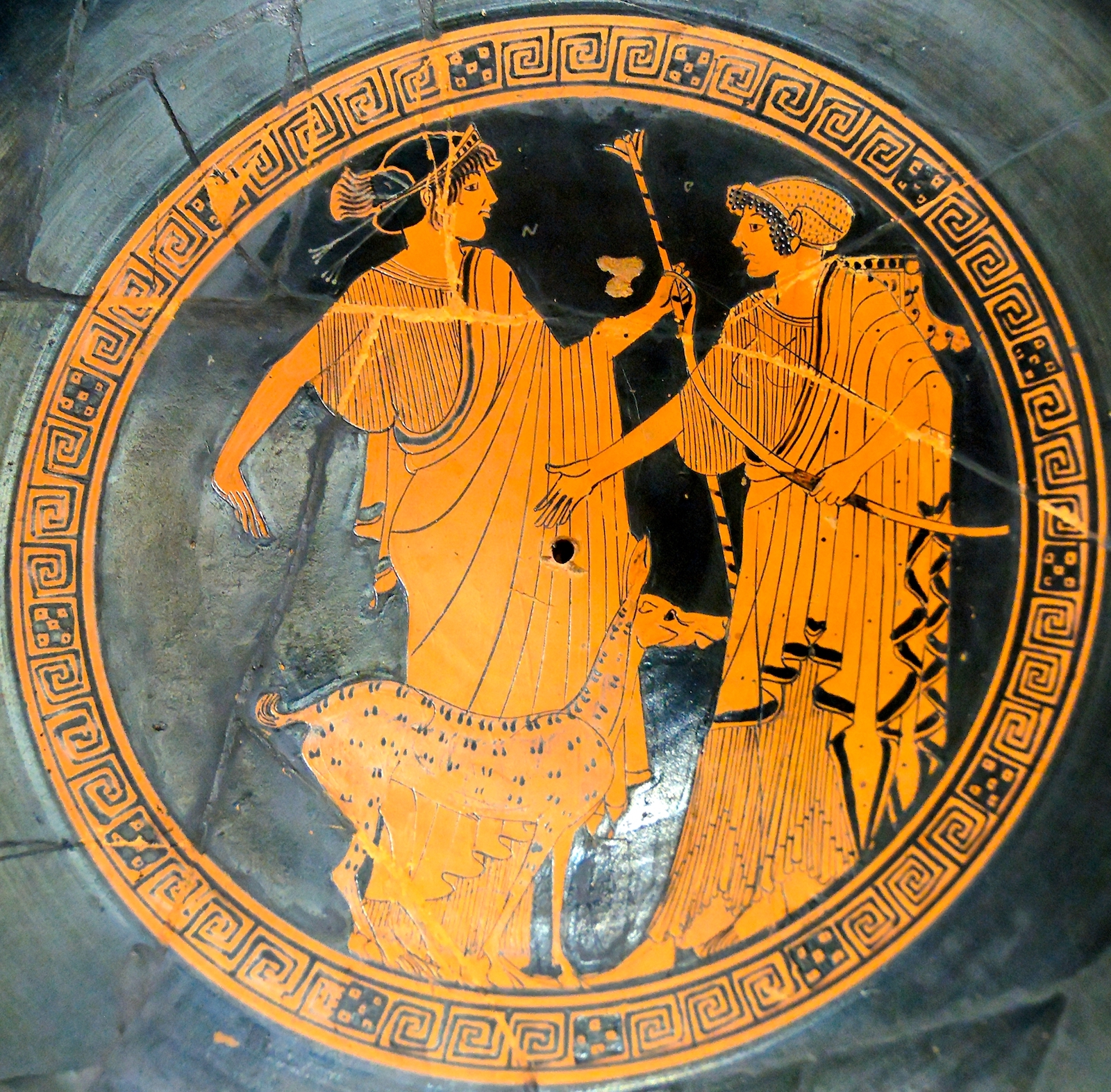
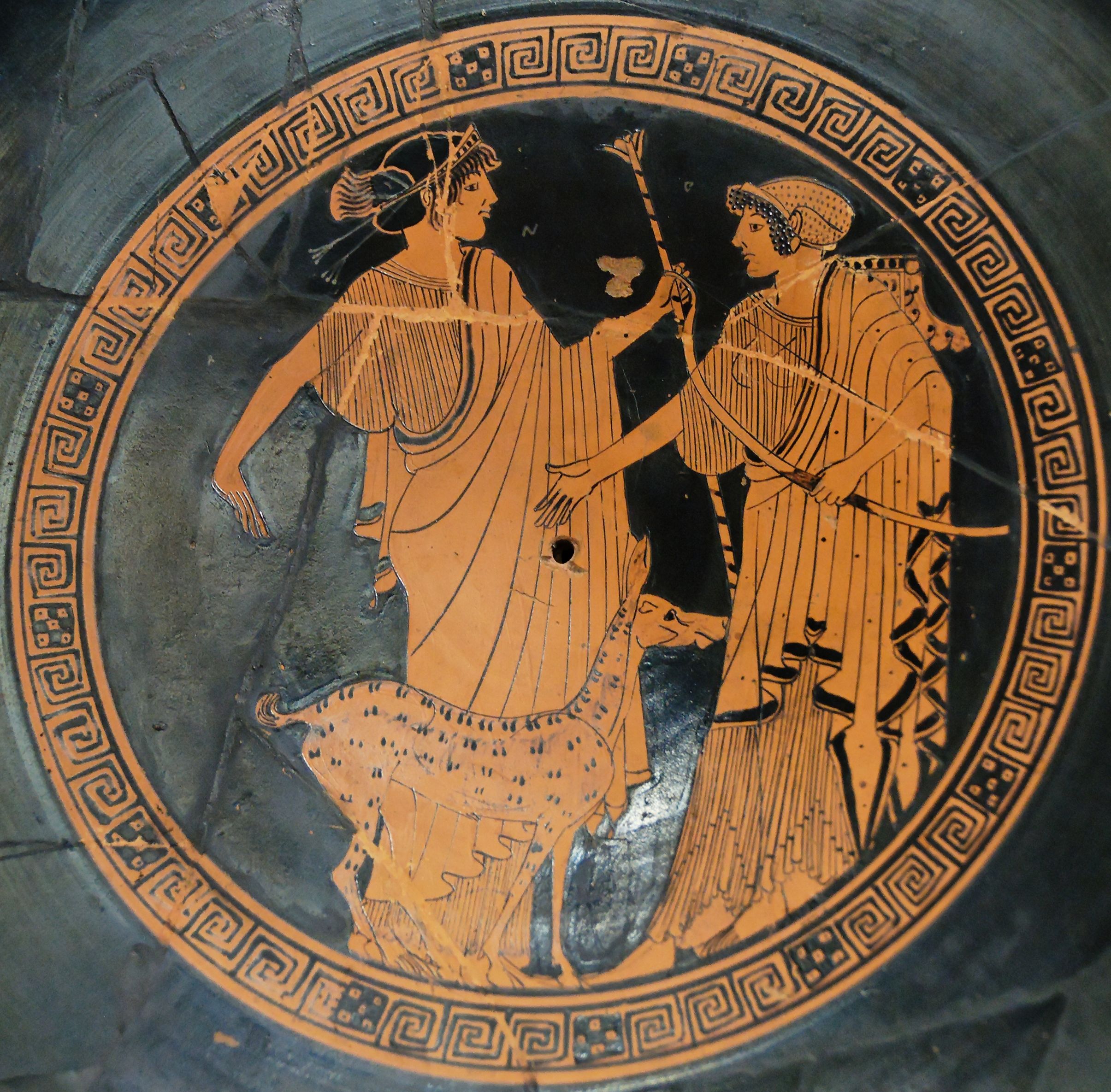
By the way, like the subjects of entropy and energy, also the subject of Apollo and Artemis is very classical as this pottery (dated around 490-470 BC) of Brygos shows: (source.) Brygos must have been a contemporary of Pythagoras (570-495 BC) Its amazing how well the pottery has survived the 2500 years. Unfortunately the real name of the Brygos painter is unknown.

 = \chi(G)")