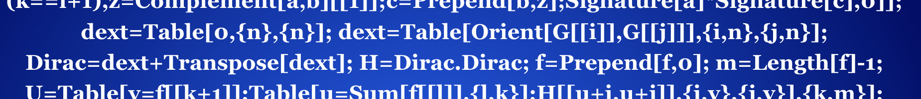
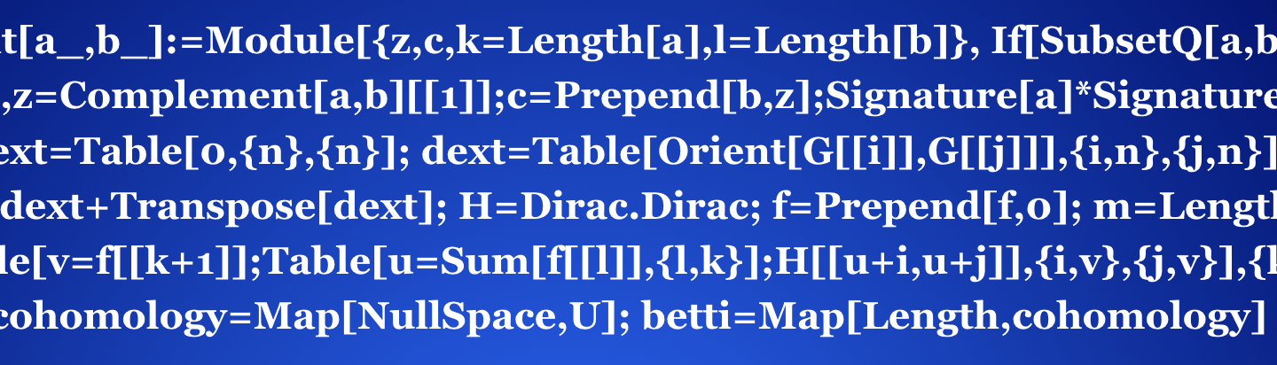
Here is the code to compute a basis of the cohomology groups of an arbitrary simplicial complex. It takes 6 lines in mathematica without any outside libraries.
The input is a simplicial complex, the out put is the basis for $H^0,H^1,H^2 etc$. The length of the code compares in complexity with computations in basic planimetric computations in a triangle (Example [mathematica notebook] for Math E320). We just compute the Dirac operator D, then split up the blocks Hk of D2 and compute their kernel. These vector spaces are now equivalent to the cohomology groups by Hodge.The genious move of Hodge is that rather than talking about equivalence classes of cocycles (which requires some mathematical training to appreciate), one can look at the kernel of concrete matrices (which we do after three weeks in an intro course of linear algebra). In the following self contained code, the first 4 lines generate a random simplicial complex. Then, in the next 6 lines, the Dirac and Hodge operator is computed. Finally, the basis of the null spaces of the Laplacians are spit out). The cohomology in the discrete has again and again been reinvented, but it is definitely due to Betti or Poincare, the key idea being the notion of the incidence matrix d, which implements “div, grad, curl etc”.
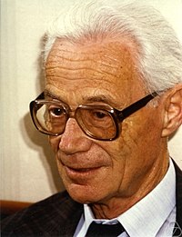
The earliest reference for discrete Hodge I could find is the survey lecture “The {Euler} characteristic – a few highlights in its long history” by Benno Eckmann. As a graduate student, I have seen one one of these survey lectures, and it had been the one about Euler characteristic. The talk was brilliant and the lecture hall at the nearby university had been packed. I never took a course from Eckmann, he got retired, but Eckmann was still seen a lot at the department when I was a student there. He had been the person who told me that I won the fellowship to spend a year in Israel (1988-1989). The following code shows also that the topic of cohomology is something which could be introduced early on in a linear algebra course as it is just the process of computing the kernel of a specific matrix. We just had covered that in our linear algebra course Math 21b.
Generate[A_]:=Delete[Union[Sort[Flatten[Map[Subsets,A],1]]],1]
R[n_,m_]:=Module[{A={},X=Range[n],k},Do[k:=1+Random[Integer,n-1];
  A=Append[A,Union[RandomChoice[X,k]]],{m}];Generate[A]];
G=R[10,16];n=Length[G]; Dim=Map[Length,G]-1;f=Delete[BinCounts[Dim],1];
Orient[a_,b_]:=Module[{z,c,k=Length[a],l=Length[b]}, If[SubsetQ[a,b] &&
(k==l+1),z=Complement[a,b][[1]];c=Prepend[b,z];Signature[a]*Signature[c],0]];
dext=Table[0,{n},{n}]; dext=Table[Orient[G[[i]],G[[j]]],{i,n},{j,n}];
Dirac=dext+Transpose[dext]; H=Dirac.Dirac; f=Prepend[f,0]; m=Length[f]-1;
U=Table[v=f[[k+1]];Table[u=Sum[f[[l]],{l,k}];H[[u+i,u+j]],{i,v},{j,v}],{k,m}];
cohomology=Map[NullSpace,U]; betti=Map[Length,cohomology]
You can see why there is a lot of theory to compute the cohomology more effectively. A computer does not mind to find the kernel of large matrices, but when dealing with simplicial complexes with thousands of elements, then the computer has to work hard too.
By the way, various Dirac operators have been considered in the discrete. It appears that discrete Dirac operator as a matrix in the discrete had been overlooked for long. The Dirac operator in the continuum is a silly beast as one has to use a Clifford algebra in order to factor the Laplacian. In the discrete, such gymnastics is not unnecessary. But it is nice. McKean-Singer for example is quite simple in the discrete, when following the approach of the Cycon-Froese-Kirsch and Simon book (the later book had been one of the key books for me in graduate school).