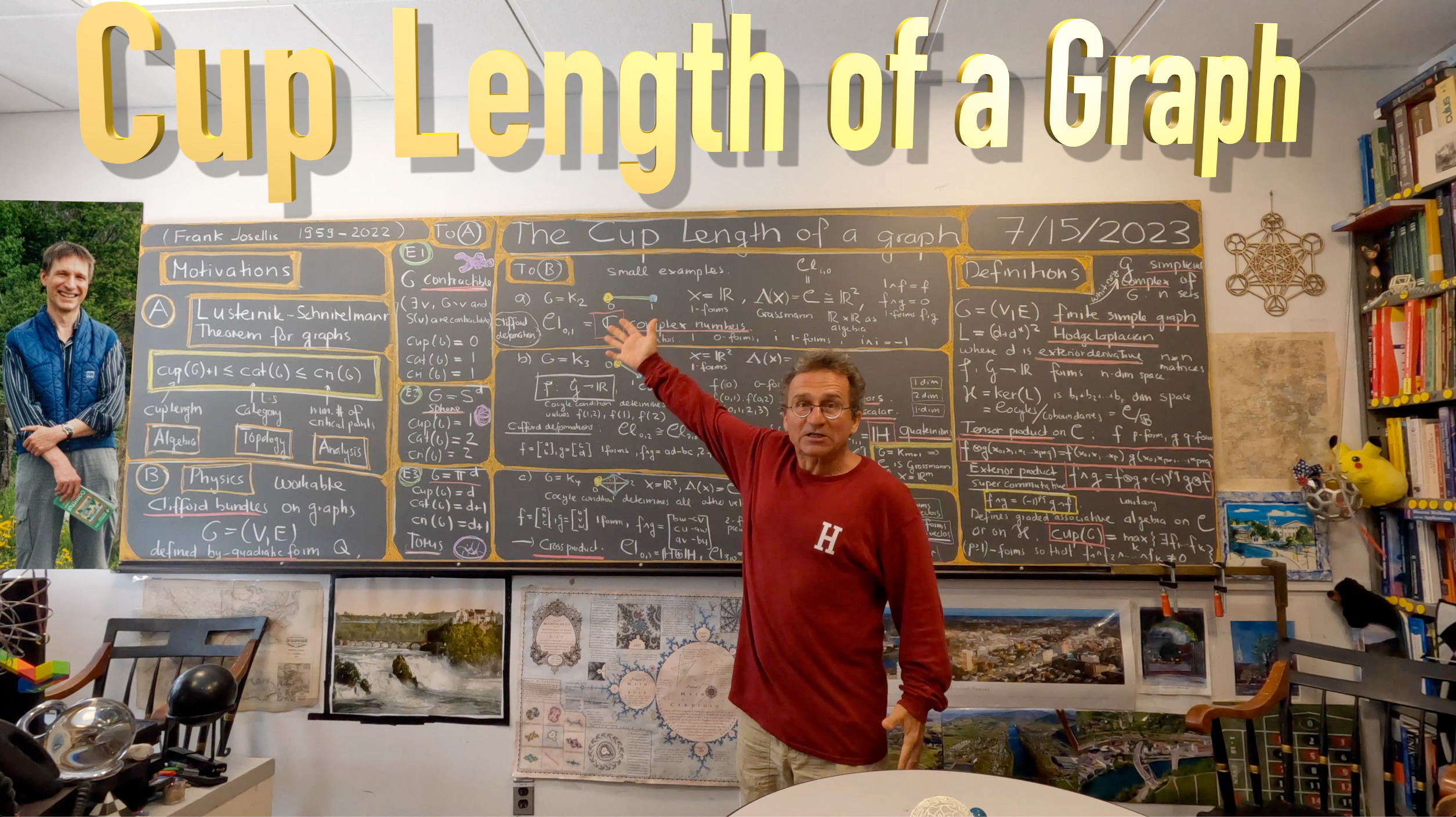
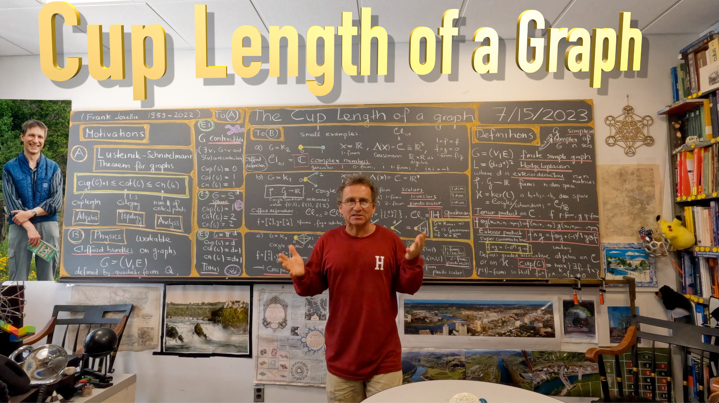
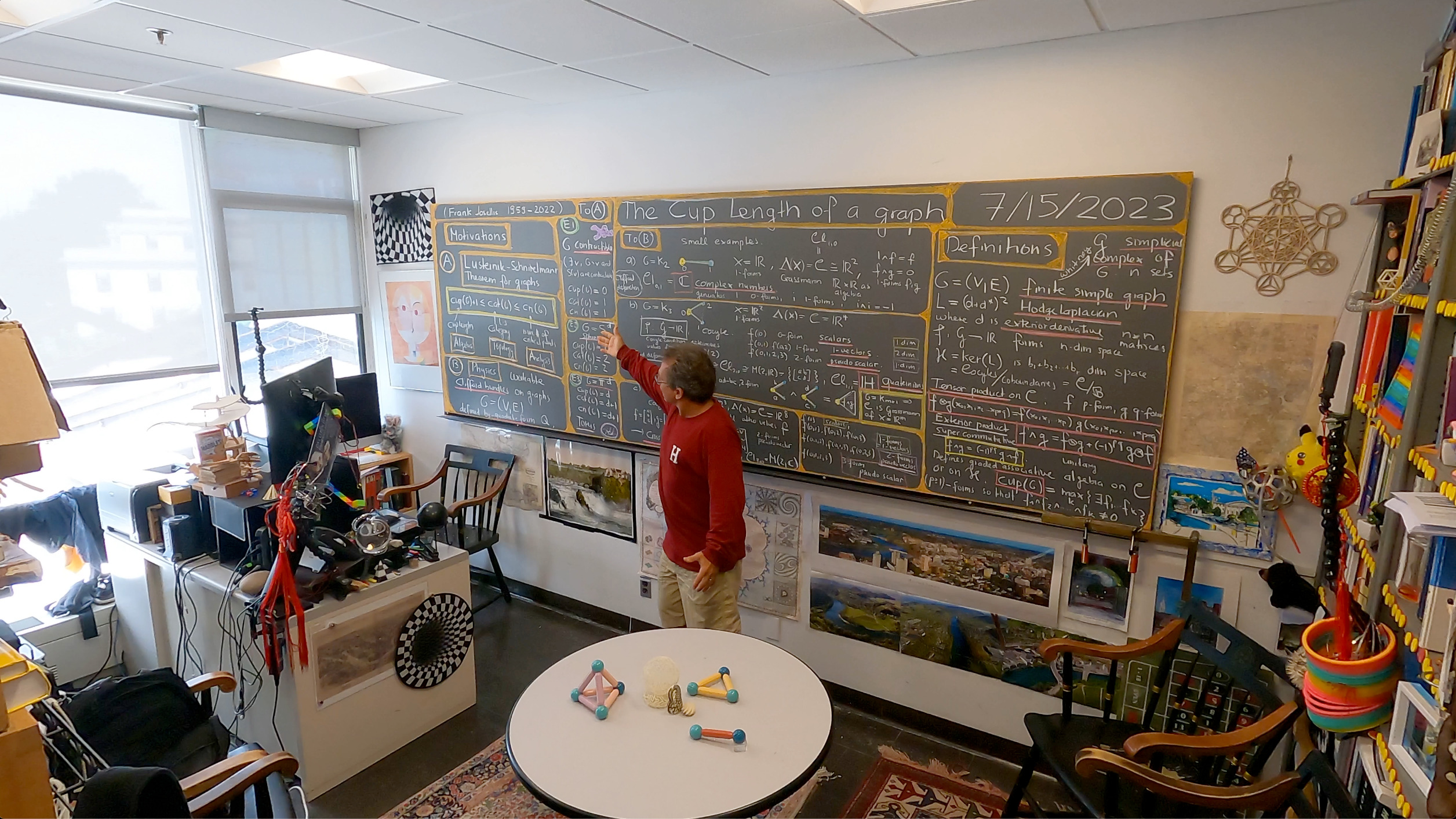
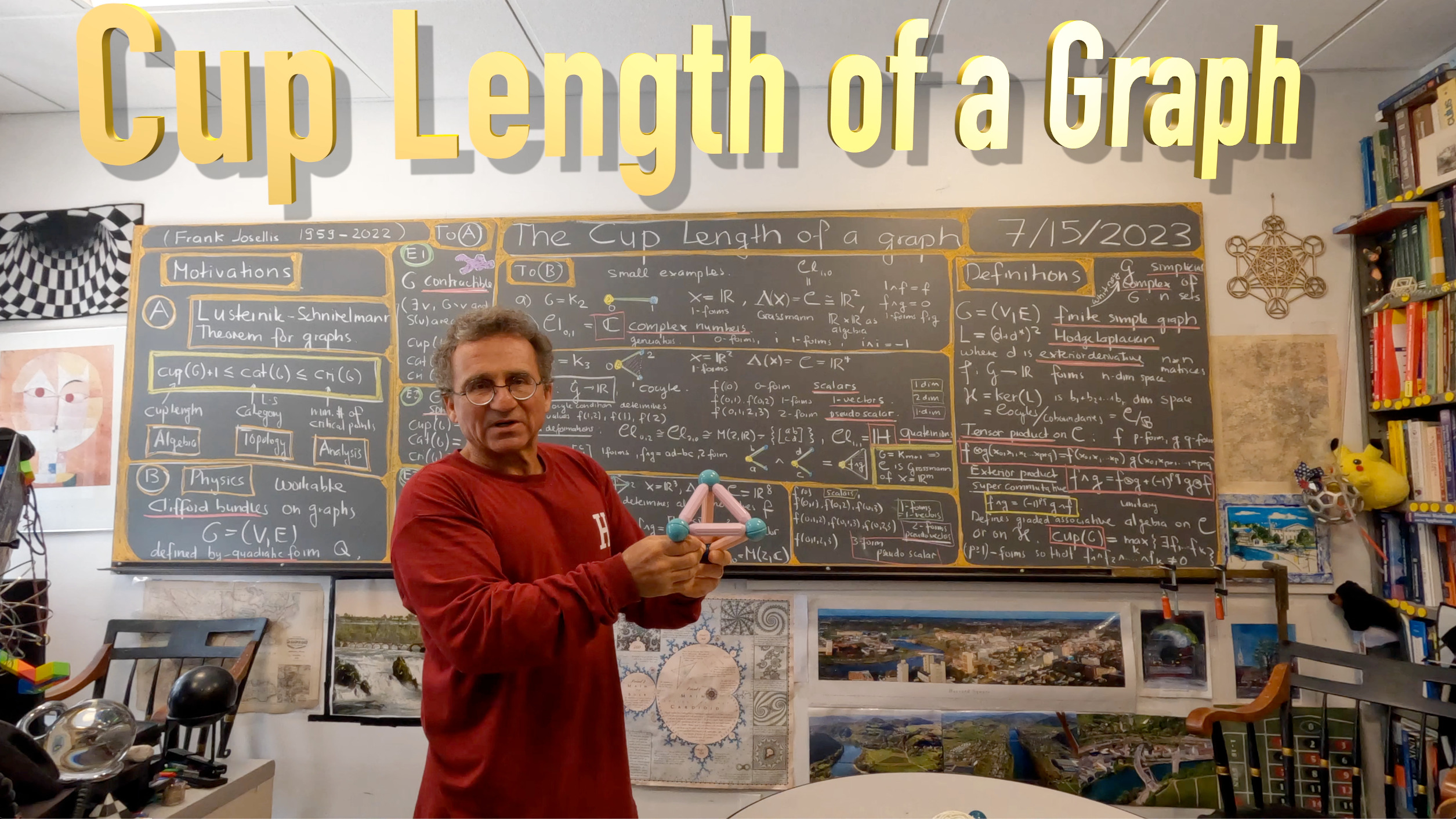
Finite geometry appears to be remote to Euclidean spaces. In reality it is very close, if one uses the right definitions. Basic questions are 1) How natural are the definitions 2) How do theorems look like 3) how difficult are the proofs. Lusternik-Schnirelmann theory like its sibling Morse theory is an ideal test ground. It turns out that the definitions are not only easier, the proofs are much more transparent and the theorems have identical statements. I worked on this project with Frank Josellis in 2012 (here is the preprint) which needs a bit of revision. It was written at a time, many other topics awaited work after (Gauss Bonnet and Poincare Hopf and Brouwer-Lefshetz in the discrete just happened for graphs) and there was so much other geometry to be done (and still is today a lot of work remains to be done). 2012 also still was a time, where almost everybody (especially graph theorists) still looked at graphs as one dimensional simplicial complexes. Lusternik-Schnirelmann theory is a wonderful topic because it is a place, where Algebra, Topology and Analysis touch in a single simple inequality . The cup length is defined as in the continuum as the maximal number of positive degree cohomology classes which when multiplied give a non-zero cohomology class. The category is the minimal of contractible graphs covering the graph. The number cri(G) is the minimal number of critical points which a locally injective function can have on the graph. This is in general smaller than the number of critical points which a Morse function can have. On a 2-torus for example, the minimal number of critical points is 3 while the minimal number of Morse critical points is 4. The key for the cup length is to define an algebra structure on the linear space of cohomology classes and so get a cohomology ring. Hodge theory allows to see the vector space of cohomology classes as the kernel of a single matrix L, defined by the graph G (or rather its natural simplicial complex). There is a natural functor from graphs to simplicial complexes which assigns to a graph the set of subsets of complete graphs. There is a similar functor which assigns to a vector space its exterior algebra. The functor ${\rm graphs} \rightarrow {\rm simplicial \; complexes}$ is named after Hasssler Whitney, the functor is named after Hermann Grassmann. Grasssmann was the first who fleshed out the notion of linear space and its exterior algebra . Whitney was the first who saw the potential of graph theory for describing rather general topological spaces like smooth manifolds. Whitney also was able to find simple definitions. Like the fundamental conundrums which you face when looking a discrete differential forms [which are just functions on complete subgraphs, so that if you have n complete subgraphs, then we have a n-dimensional space. The functions on vertices are the scalar functions, the functions on edges are the 1-vector fields (1-forms), functions on triangles are 2-vector fields (2-forms) etc.] Whitney saw (or formulated as the first) the difficulty that if you define a tensor product of a p-form with a q-form, then you have to match a function of (p+1) variables with a function of (q+1) variables to get a function of (p+q+1) variables. Defining obviously does not work because . You would get a – form and not a – form. What one can do in the case when taking the Shannon product of two graphs is to apply the divergence operator to the tensor product which also brings the degree down by one. This actually works very well and shows that the tensor product of forms produces a differential form with the correct dimension on the product of the two graphs. The Kuenneth formula for cohomology is then very easy. When we look however at the problem to define a tensor product within ONE graph, where f,g are p respectively q forms on the same graph, we can not proceed as such. What you can do however (and I think this was implicit in Whitney’s work) is to select out a base point of a simplex and to define . Once one has a tensor product, one can get the exterior product by applying the symmetrization as in the continuum so that we have the super commutativity which means that the sign changes only if both are Fermions, meaning odd degrees. If one of them is a Boson, then we have commutativity. In the talk explain a bit how to think about this. Since we all live in the familar 3 dimensional space, let us consider a complete graph G with 4 vertices with special point . The linear space of cocycles of this graph has dimension 8 because giving the function f on determines the function values at all vertices because the cocycle condition tells that . This settles the dimension of the 0-forms, the scalars. Lets look at the 1-forms f which are the 1-vectors. There are 6 edges in the graph but the function values are all we need. For example . The vector space of 1-forms is 3 dimensional. Similarly, the vector space of 2-vectors is 3 dimensional as the values on the triangles determine the values on the 4th triangle. An then there is the pseudo scalar, the function . We see
The vector space on all cocycles of has dimension . The exterior product defined with produces an algebra which is the exterior algebra of .
For example, if is a 1-vector and is a 1-vector then is a 2-vector on the triangles. If we attach this value to the third edge not containing the triangle, we get again a 1-vector. It is the cross product of the two 1-vectors. We do not have to reinvent the wheel in the discrete. The math is the same. Interesting becomes the story when we look at p-form bundles on more general graphs. For us, however at this point is only the task to build from the cohomology space a cohomology ring.
Here is some mathematica code illustrating how we can compute the cup length: we take a concrete graph, a discrete 2 torus with Betti vector b=(1,2,1). The kernel of the matrix LL is the cohomology space. The procedure Grassmannian produces the multiplication in that space and so produces a cohomology ring. The cup length is 2 because we can find two 1-forms whose product is not zero. It can not be three as there are no 3-forms in a 2 dimensional space.
Closure[A_]:=If[A=={},{},Delete[Union[Sort[Flatten[Map[Subsets,A],1]]],1]];
F[G_]:=Module[{l=Map[Length,G]},If[G=={},{},
 Table[Sum[If[l[[j]]==k,1,0],{j,Length[l]}],{k,Max[l]}]]];
s[x_]:=Signature[x];L=Length;
s[x_,y_]:=If[SubsetQ[x,y]&&(L[x]==L[y]+1),s[Prepend[y,Complement[x,y][[1]]]]*s[x],0];
Dirac[G_]:=Module[{f=F[G],b,d,n=Length[G]},
 b=Prepend[Table[Sum[f[[l]],{l,k}],{k,Length[f]}],0];
 d=Table[s[G[[i]],G[[j]]],{i,n},{j,n}]; {d+Transpose[d],b}];
Grassmannian[G_,f_,g_]:=Module[{n=Length[G],x,y,z,i,j,p,q,v},
Table[ x=G[[k]]; m=Length[x]; Sum[ q=m-1-p; v=x[[1]];
  y=Prepend[Table[x[[j]],{j,2,p+1}],v]; z=Prepend[Table[x[[j]],{j,p+2,m}],v];
  i=First[First[Position[G,y]]];        j=First[First[Position[G,z]]];
  f[[i]]*g[[j]]-(-1)^((p+1)*(q+1))*f[[j]]*g[[i]],{p,1,m-2}], {k,n}]];
G = twotorus={{1},{2},{3},{4},{5},{6},{7},{8},{9},{10},{11},{12},{13},
{14},{15},{16},{1,2},{1,4},{1,5},{1,6},{1,13},{1,16},{2,3},{2,6},
{2,7},{2,13},{2,14},{3,4},{3,7},{3,8},{3,14},{3,15},{4,5},{4,8},
{4,15},{4,16},{5,6},{5,8},{5,9},{5,10},{6,7},{6,10},{6,11},{7,8},
{7,11},{7,12},{8,9},{8,12},{9,10},{9,12},{9,13},{9,14},{10,11},
{10,14},{10,15},{11,12},{11,15},{11,16},{12,13},{12,16},{13,14},
{13,16},{14,15},{15,16},{1,2,6},{1,2,13},{1,4,5},{1,4,16},{1,5,6},
{1,13,16},{2,3,7},{2,3,14},{2,6,7},{2,13,14},{3,4,8},{3,4,15},
{3,7,8},{3,14,15},{4,5,8},{4,15,16},{5,6,10},{5,8,9},{5,9,10},
{6,7,11},{6,10,11},{7,8,12},{7,11,12},{8,9,12},{9,10,14},{9,12,13},
{9,13,14},{10,11,15},{10,14,15},{11,12,16},{11,15,16},{12,13,16}};
n=Length[G]; DD=First[Dirac[G]];  (* Dirac operator *)
LL=DD.DD;  (* Hodge Laplacian *)
NS=NullSpace[LL];   (*a basis for the cohomology ring *)
f = NS[[2]]; g = NS[[3]];
Grassmannian[G, f, g]            (* this is the cup product of the two 1-forms *)
NS[[1]]                                    (* this is the volume form. It is the same      *)
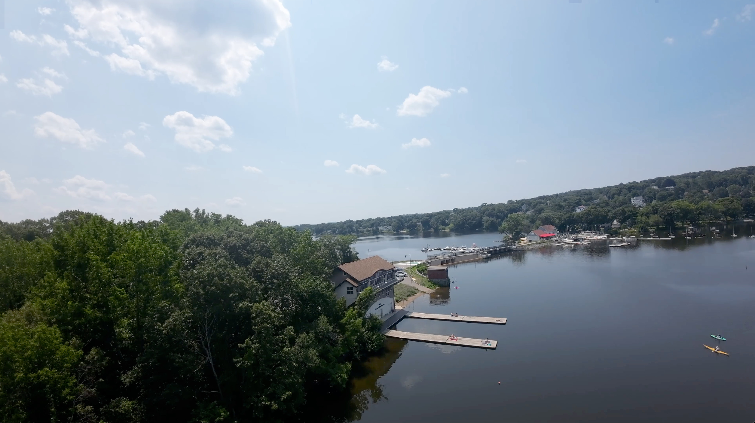
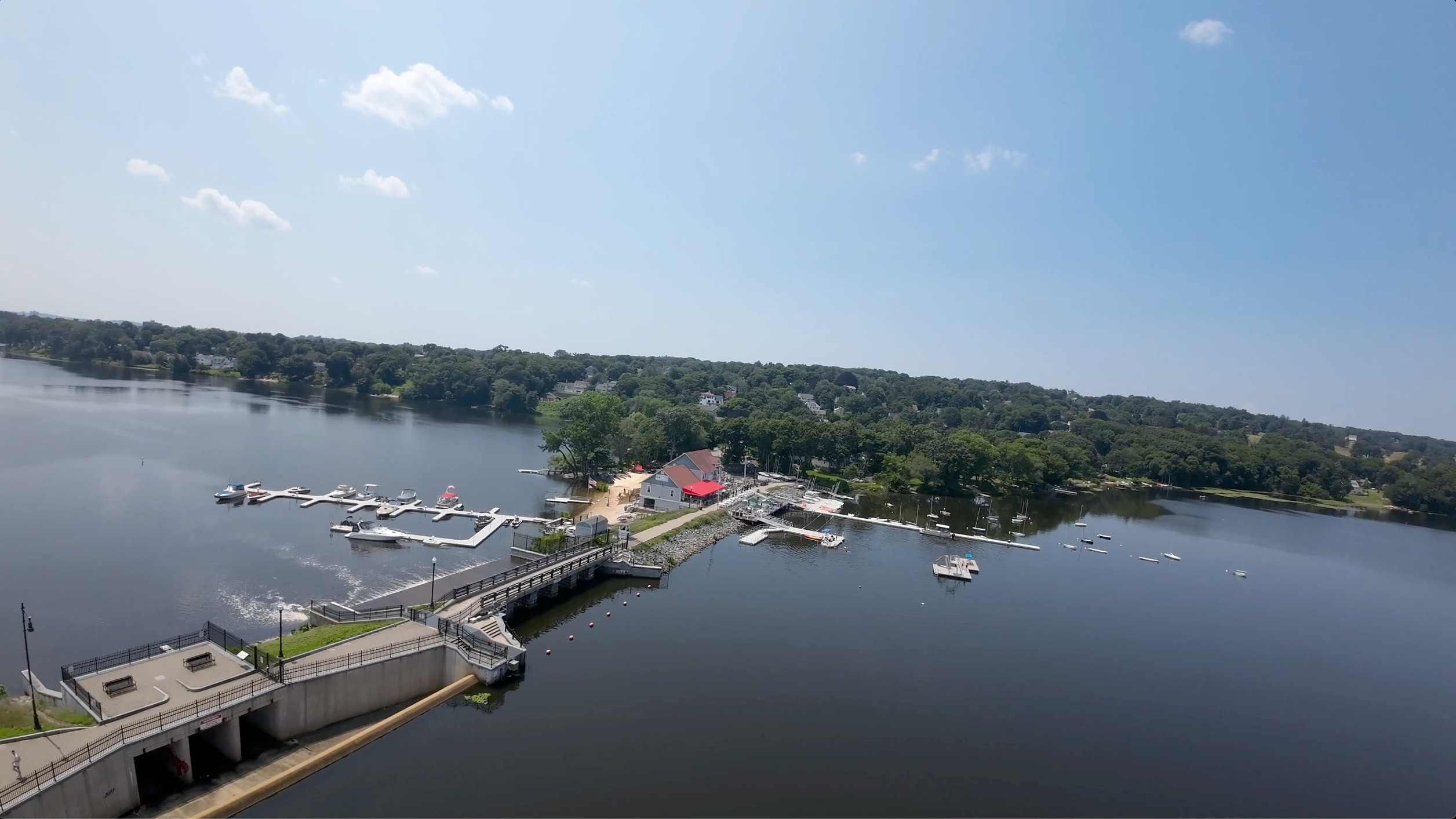
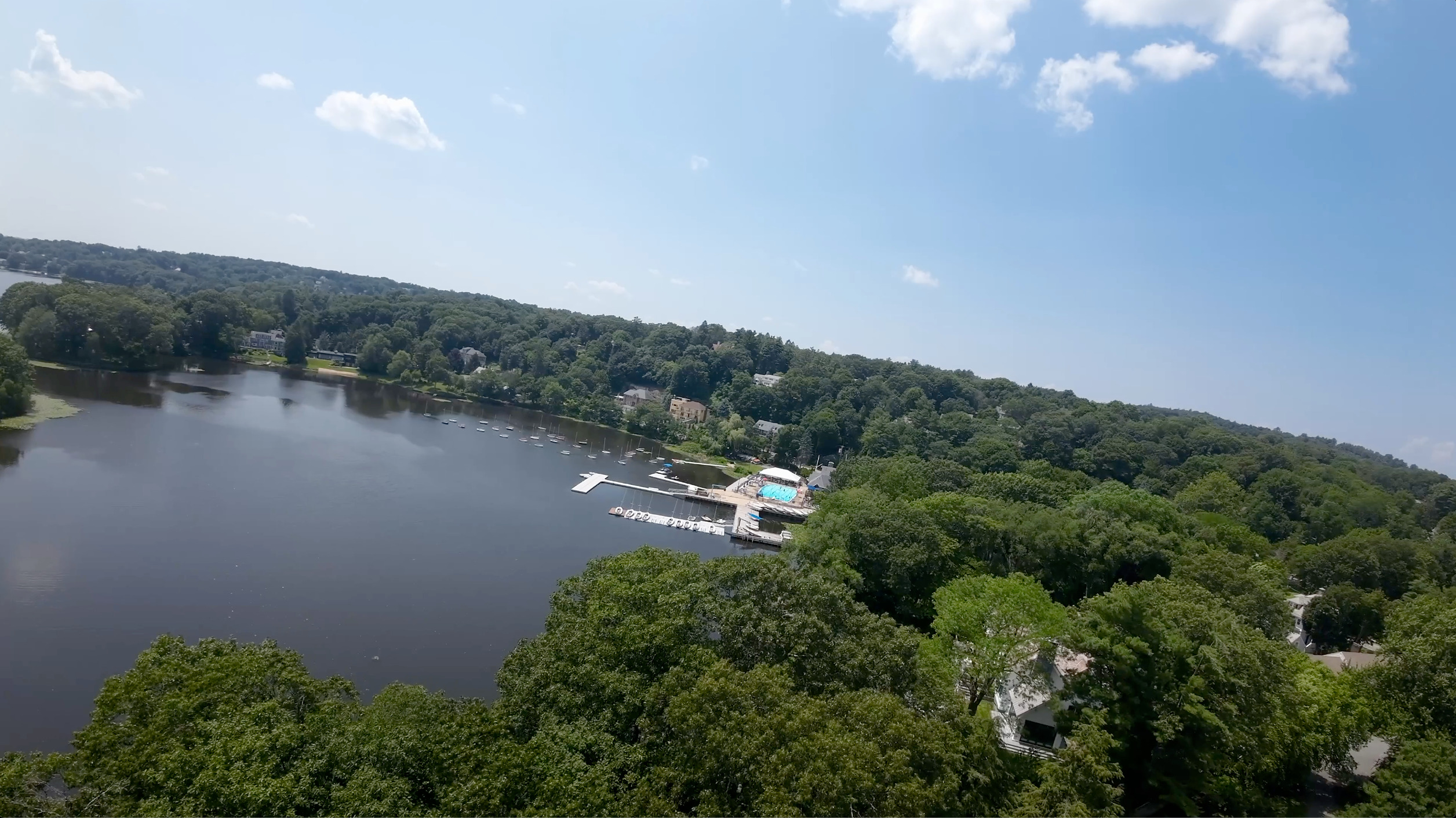
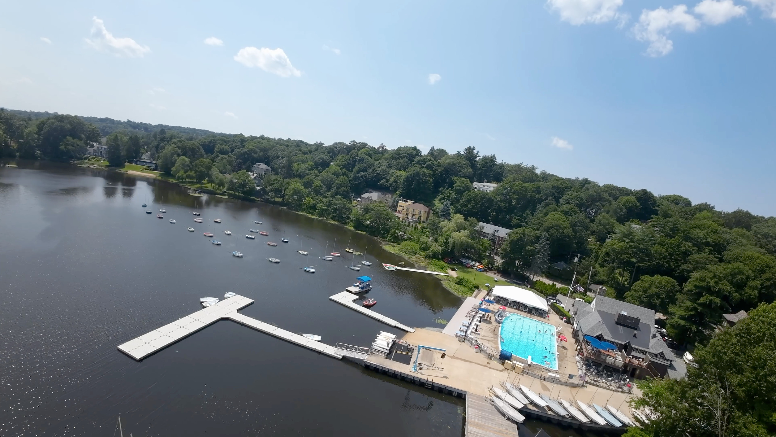
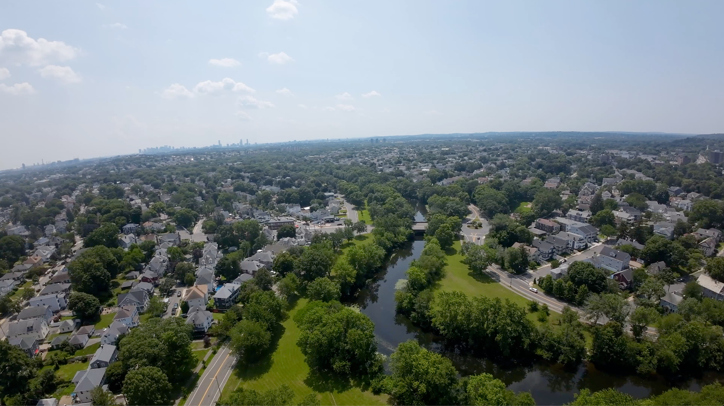
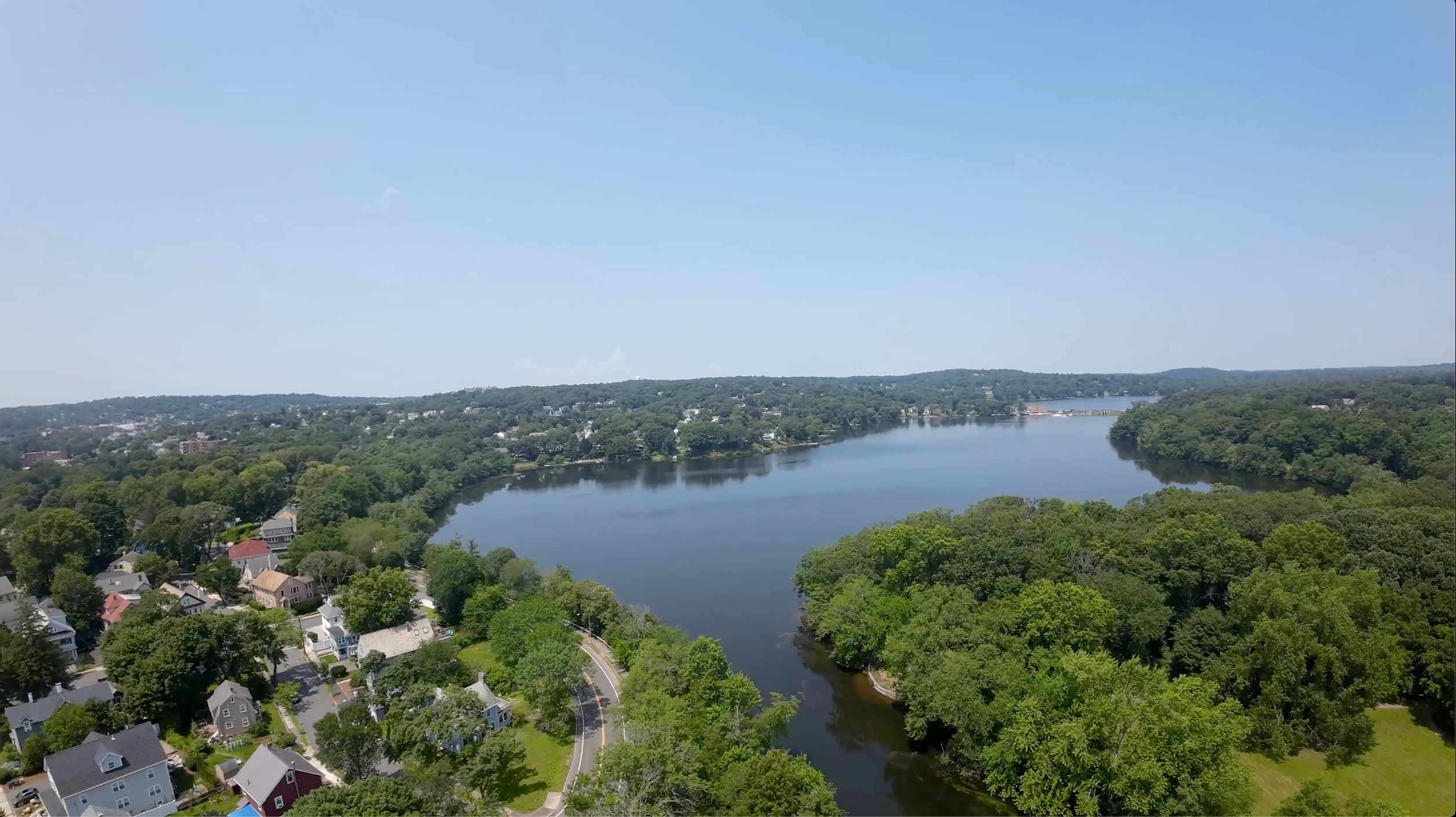
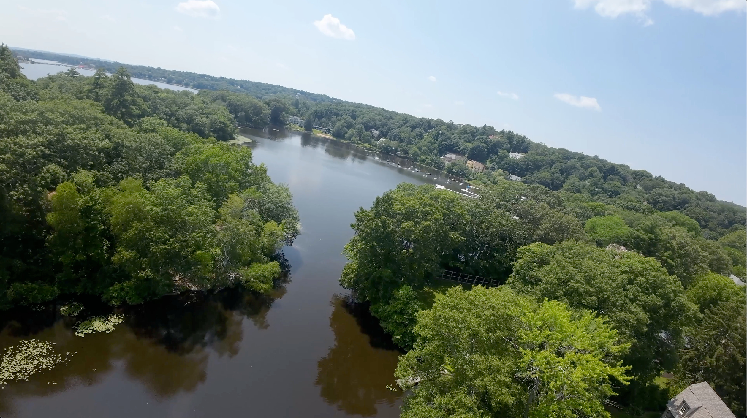
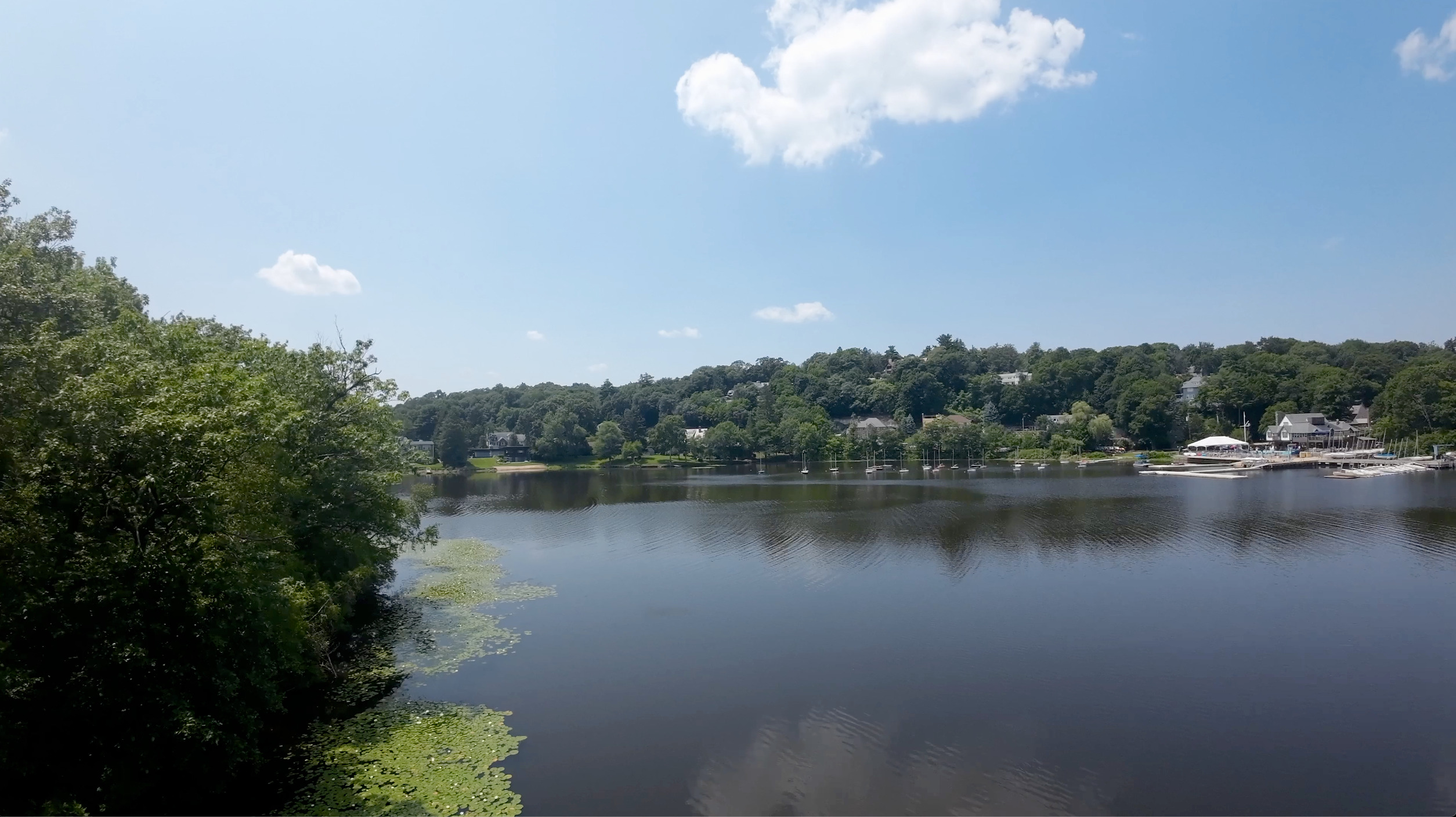
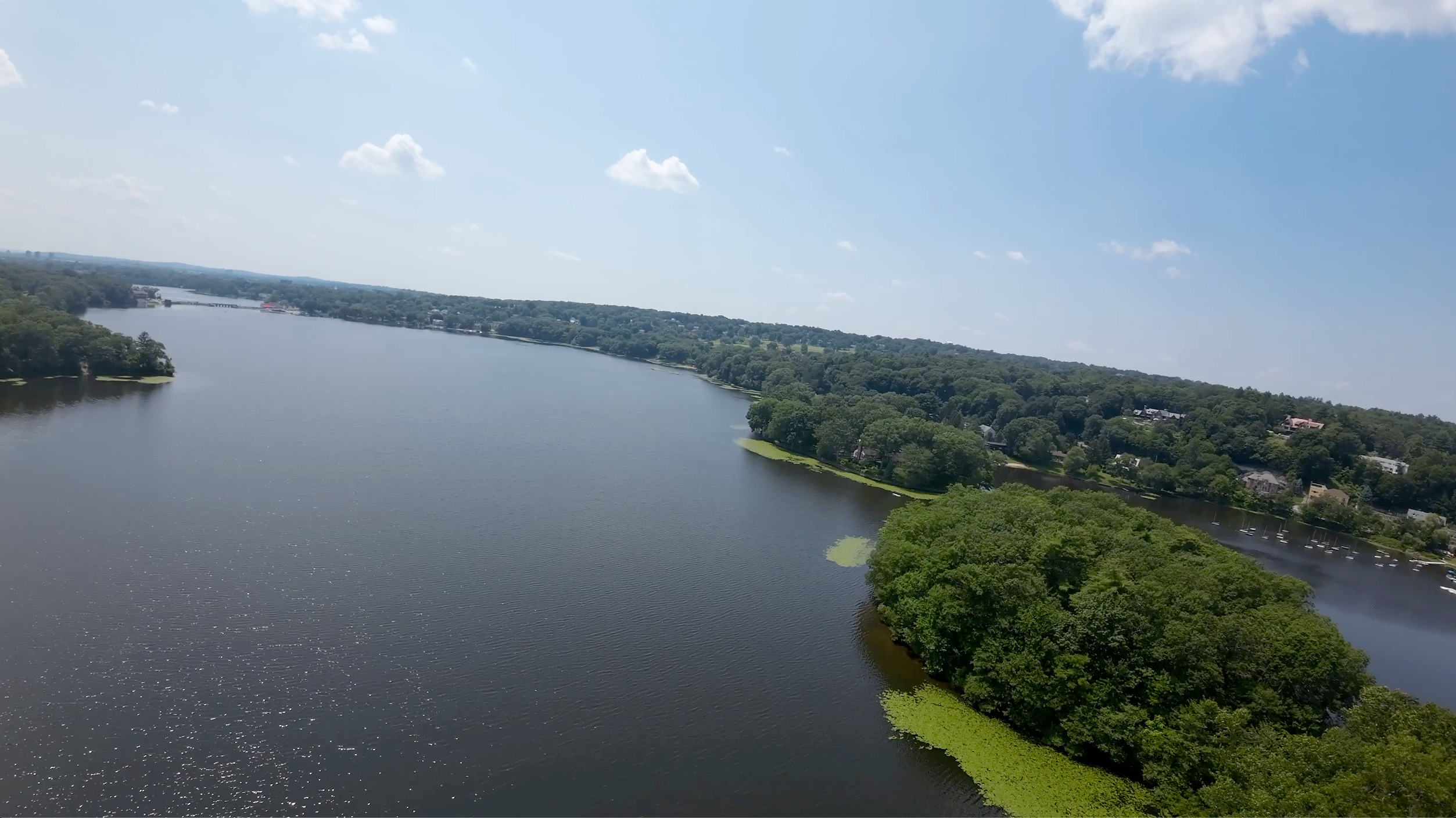
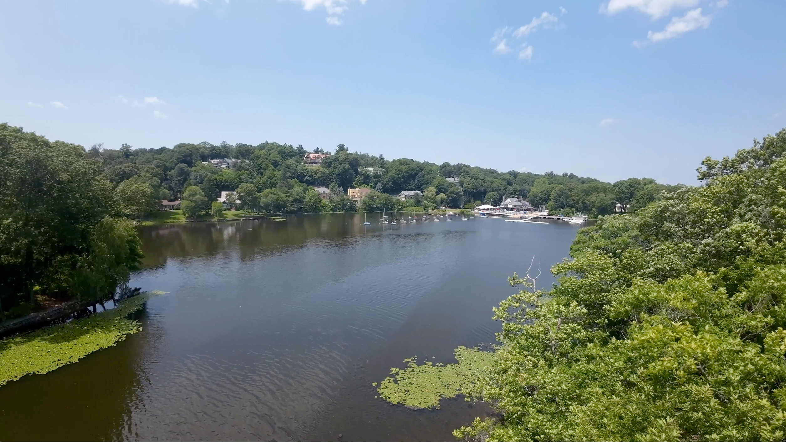
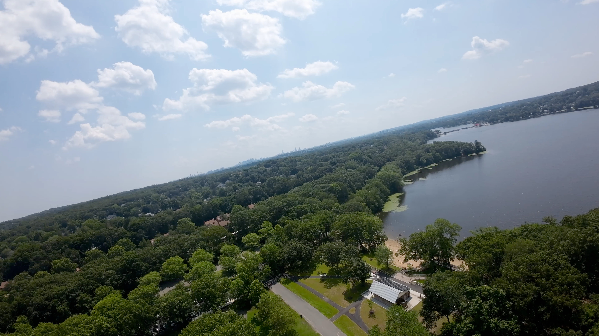
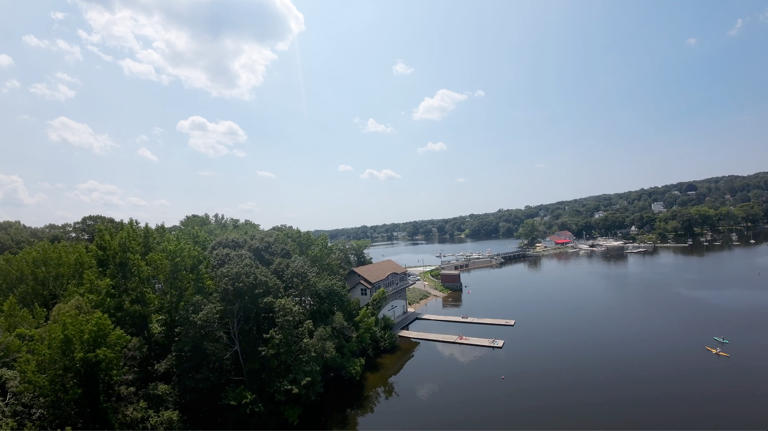
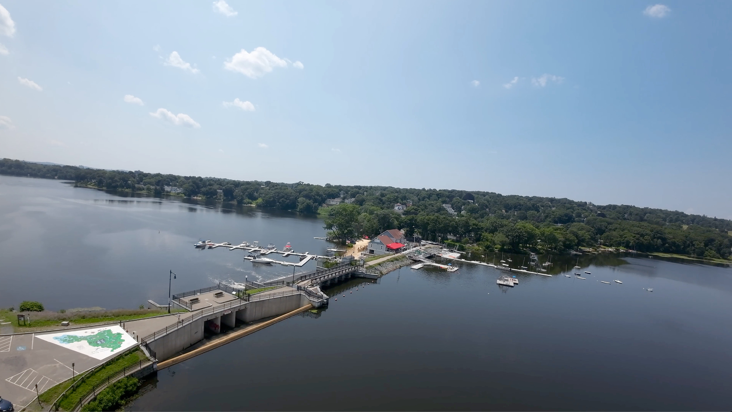
Medford Boat clubtDam between upper and lower Mystic riverWinchester boat clubWinchester Boat clubThe middlesex canal passed hereScreenshotScreenshotScreenshotScreenshotScreenshotScreenshotScreenshotThis is the passage where the middlesex canal passed ScreenshotScreenshotScreenshotShannon beach in MedfordTufts sailing house and Medford boat clubMedford boat club
 +1 \leq cat(G) \leq cri(G)")
")


 = f(x_1, \dots x_q) g(x_{p+1} .. x_{p+q+1})")
 \neq p+q+1")
")
")


 = f(x_0,x_1, \dots x_q) g(x_0,x_{p+1} .. x_{p+q})")
^{p q} g \otimes f")
^{p q} g \wedge h")


 = \nabla f(x_0,x_k) = f(x_k)-f(x_0)=0")
 = f_{x_0}")
,b=f(x_0,x_2),c=f(x_0,x_3)")
 = f(x_1,x_0) + f(x_0,x_2)")
, f(x_0,x_2,x_3), f(x_0,x_3,x_1)")
")


![f=[a,b,c]](https://s0.wp.com/latex.php?latex=f%3D%5Ba%2Cb%2Cc%5D&bg=ffffff&fg=000000&s=0 "f=[a,b,c]")
![[u,v,w]](https://s0.wp.com/latex.php?latex=%5Bu%2Cv%2Cw%5D&bg=ffffff&fg=000000&s=0 "[u,v,w]")
![[a,b,c] \wedge [u,v,w]](https://s0.wp.com/latex.php?latex=%5Ba%2Cb%2Cc%5D+%5Cwedge+%5Bu%2Cv%2Cw%5D&bg=ffffff&fg=000000&s=0 "[a,b,c] \wedge [u,v,w]")