[Update May 29, 2017:] Paper [PDF] on this has been posted now. It also includes Mathematica code, where everything can be tried out. Its so short, why not post it here too. You can experiment with the main result equating the hydrogen trace with the generating function or then with the sphere characteristic curvatures.
UnitSphere[s_,a_]:=Module[{b=NeighborhoodGraph[s,a]},
  If[Length[VertexList[b]]<2,Graph[{}],VertexDelete[b,a]]];
UnitSpheres[s_]:=Map[Function[x,UnitSphere[s,x]],VertexList[s]];
F[A_,z_]:=A-z IdentityMatrix[Length[A]]; F[A_]:=F[A,-1];
FredholmDet[s_]:=Det[F[AdjacencyMatrix[s]]];
BowenLanford[s_,z_]:=Det[F[AdjacencyMatrix[s],z]];
CliqueNumber[s_]:=Length[First[FindClique[s]]];
ListCliques[s_,k_]:=Module[{n,t,m,u,r,V,W,U,l={},L},L=Length;
  VL=VertexList;EL=EdgeList;V=VL[s];W=EL[s]; m=L[W]; n=L[V];
  r=Subsets[V,{k,k}];U=Table[{W[[j,1]],W[[j,2]]},{j,L[W]}];
  If[k==1,l=V,If[k==2,l=U,Do[t=Subgraph[s,r[[j]]];
  If[L[EL[t]]==k(k-1)/2,l=Append[l,VL[t]]],{j,L[r]}]]];l];
Whitney[s_]:=Module[{F,a,u,v,d,V,LC,L=Length},V=VertexList[s];
  d=If[L[V]==0,-1,CliqueNumber[s]];LC=ListCliques;
  If[d>=0,a[x_]:=Table[{x[[k]]},{k,L[x]}];
  F[t_,l_]:=If[l==1,a[LC[t,1]],If[l==0,{},LC[t,l]]];
  u=Delete[Union[Table[F[s,l],{l,0,d}]],1]; v={};
  Do[Do[v=Append[v,u[[m,l]]],{l,L[u[[m]]]}],{m,L[u]}],v={}];v];
Barycentric[s_]:=Module[{v={},c=Whitney[s]},Do[Do[If[c[[k]]!=c[[l]]
  && (SubsetQ[c[[k]],c[[l]]] || SubsetQ[c[[l]],c[[k]]]),
  v=Append[v,k->l]],{l,k+1,Length[c]}],{k,Length[c]}];
  UndirectedGraph[Graph[v]]];
ConnectionGraph[s_] := Module[{c=Whitney[s],n,A},n=Length[c];
  A=Table[1,{n},{n}];Do[If[DisjointQ[c[[k]],c[[l]]]||
  c[[k]]==c[[l]],A[[k,l]]=0],{k,n},{l,n}];AdjacencyGraph[A]];
ConnectionLaplacian[s_]:=F[AdjacencyMatrix[ConnectionGraph[s]]];
FredholmCharacteristic[s_]:=Det[ConnectionLaplacian[s]];
GreenF[s_]:=Inverse[ConnectionLaplacian[s]];
Energy[s_]:=Total[Flatten[GreenF[s]]];
BarycentricOp[n_]:=Table[StirlingS2[j,i]i!,{i,n+1},{j,n+1}];
Fvector[s_] := Delete[BinCounts[Length /@ Whitney[s]], 1];
Fvector1[s_]:=Module[{f=Fvector[s]},BarycentricOp[Length[f]-1].f];
Fv=Fvector; Fv1=Fvector1;
GFunction[s_,x_]:=Module[{f=Fv[s]},1+Sum[f[[k]]x^k,{k,Length[f]}]];
GFunction1[s_,x_]:=Module[{f=Fv1[s]},1+Sum[f[[k]]x^k,{k,Length[f]}]];
dim[x_]:=Length[x]-1; Pro=Product; W=Whitney;
Euler[s_]:=Module[{w=W[s],n},n=Length[w];Sum[(-1)^dim[w[[k]]],{k,n}]];
Fermi[s_]:=Module[{w=W[s],n},n=Length[w];Pro[(-1)^dim[w[[k]]],{k,n}]];
Eta[s_]:=Tr[ConnectionLaplacian[s]-GreenF[s]];
Eta0[s_]:=Total[Map[Euler,UnitSpheres[s]]];
Eta1[s_]:=Total[Map[Euler,UnitSpheres[Barycentric[s]]]];
EtaG[s_]:=Module[{g=GFunction1[s,x]}, f[y_]:=g /. x->y;f'[0]-f'[-1]];
EulerG[s_]:=Module[{g=GFunction[s,x]},f[y_]:=g /. x->y;f[0] -f[-1] ];

s=RandomGraph[{23,60}]; sc = ConnectionGraph[s];
{Euler[s],Energy[s],EulerG[s]}
{Fermi[s],BowenLanford[sc,-1],FredholmCharacteristic[s]}
{Eta1[s],Eta[s],EtaG[s]}
Summary
The hydrogen trace of a simplicial complex is a functional which can be expressed in many different ways, algebraically as a trace, geometrically as a Gauss-Bonnet formulas or analytically as a derivative of a polynomial at a point. We believed first that it is always non-negative and that minima of this functional must be even dimensional discrete manifolds. [Update May 25: there are examples where the functional is negative]. Similarly as Wu characteristic  = \sum_{x \sim y} \omega(x) \omega(y)")
=(-1)^{dim(x)}")
 = \sum_x \omega(x)")
 = \prod_x \omega(x)")
")
=\sum_{k=1}^{\infty} v_{k-1} x^k")
")
=h(0)-h(-1)")
 = h'(0)-h'(-1)")
, \psi(G), \eta(G)")
 =\sum_x \chi(S(x))")
The hydrogen trace
Given a finite abstract simplicial complex G, we have a connection Laplacian L which is invertible. Its Green function 
")
 = 1/|x-y|")
")
 = \sum_{x,y} g(x,y)")

 = L u -V u")

 = V_x(y) = g(x,y)")
(y) = L u - g(x,y) u(y)")
(y) = L u - g u")


![H=\left[ \begin{array}{ccc}1&1&1 \\1&1&0 \\ 1&0&1 \\ \end{array}\right]](https://s0.wp.com/latex.php?latex=H%3D%5Cleft%5B+%5Cbegin%7Barray%7D%7Bccc%7D1%261%261+%5C%5C1%261%260+%5C%5C+1%260%261+%5C%5C+%5Cend%7Barray%7D%5Cright%5D&bg=ffffff&fg=000000&s=0 "H=\left[ \begin{array}{ccc}1&1&1 \\1&1&0 \\ 1&0&1 \\ \end{array}\right]")

![H=\left[ \begin{array}{ccc}2&0&0\\0&1&1\\ 0&1&1 \\ \end{array}\right]](https://s0.wp.com/latex.php?latex=H%3D%5Cleft%5B+%5Cbegin%7Barray%7D%7Bccc%7D2%260%260%5C%5C0%261%261%5C%5C+0%261%261+%5C%5C+%5Cend%7Barray%7D%5Cright%5D&bg=ffffff&fg=000000&s=0 "H=\left[ \begin{array}{ccc}2&0&0\\0&1&1\\ 0&1&1 \\ \end{array}\right]")
An Example
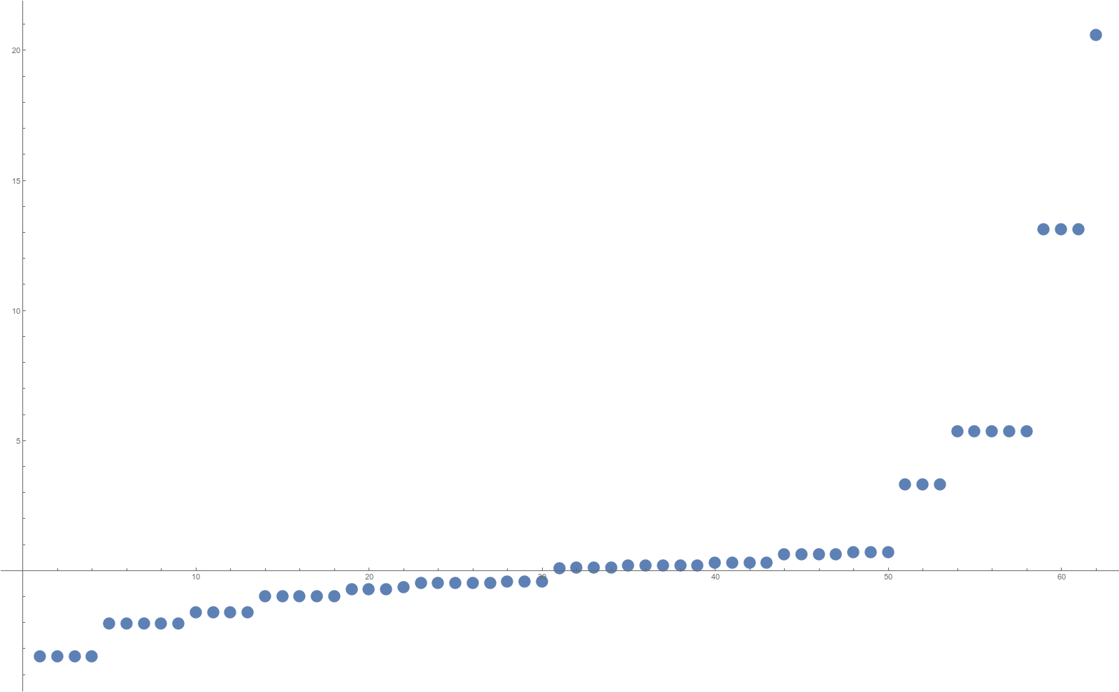
Despite some physics jargon (which we add for fun), this post is purely mathematical. It deals with a struggle to understand more about the eigenvalues of the connection Laplacian L. Unlike the Hodge Laplacian L=D2 for which we have perfect super symmetry and equal amount of negative and positive spectrum, the connection Laplacian has an asymmetry. We would like to understand that. We even want to understand whether there is always a negative eigenvalue of L. At the moment, we don’t know. But we can quantify things with measurements and related concepts. One of the main themes here is a relation to the Hydrogen Laplacian H and especially the trace of that matrix. We know that the super trace is zero, but the trace of H always appears to be non-negative. We have not yet succeeded so far to prove this. We see below the spectrum L of the connection Laplacian of the icosahedron graph, a two dimensional complex with 62 faces (f-vector is 12,30,20 as already counted by Descartes who was the first to experiment with Euler characteristic). For the Laplacian L, here are 32 positive eigenvalues and 30 negative ones. The maximal eigenvalue is 20.5807, the minimal eigenvalue is -3,30278. The Trace of the Hydrogen Laplacian H = L – L-1 is 0, an extreme case. It is related by the unit sphere theorem to the fact that all unit spheres are circles (here circular graphs C5) of Euler characteristic 0.
The Hydrogen operator H
The operator is quite interesting. We know already that for any simplicial complex G: (see this article):
| Theorem (McKean Singer) The Hydrogen Laplacian H satisfies Str(H) = 0., |
Proof. =\chi(G)")
=\chi(g)")
For the following, see this paper:
| Theorem (unit Sphere theorem) The hydrogen Laplacian satisfies Tr(H) = ∑x χ(S(x)). |
Proof. The sphere theorem assured the diagonal entries of g are )")
 = tr(L)-\sum_x \chi(S(x))")
 = tr(L)-tr(g) = \sum_x \chi(S(x))")
The hydrogen trace conjecture
Now, we have done quite a bit experiments with the Hydrogen trace Tr(H) and suspect the following:
| Hydrogen trace inequality Conjecture ([Is false]) Tr(H) ≥ 0 for all complexes with equality if and only if G is a graph for which all unit spheres have zero Euler characteristic. |
It is true for all connected graphs with less than 7 vertices. For larger graphs, we just ran it through many random graphs and so far did not find a counter example. Note that for a graph G itself it can happen that the sum of the Euler characteristic of the unit spheres is negative. But the claim is that this can not happen for graphs which are Barycentric refinements.
The functional Tr(H) appears to define therefore to be an interesting variational problem. If the above conjecture is true, then it is likely that all the minima are even dimensional geometric graphs. In some sense, the functional would select discrete manifolds.
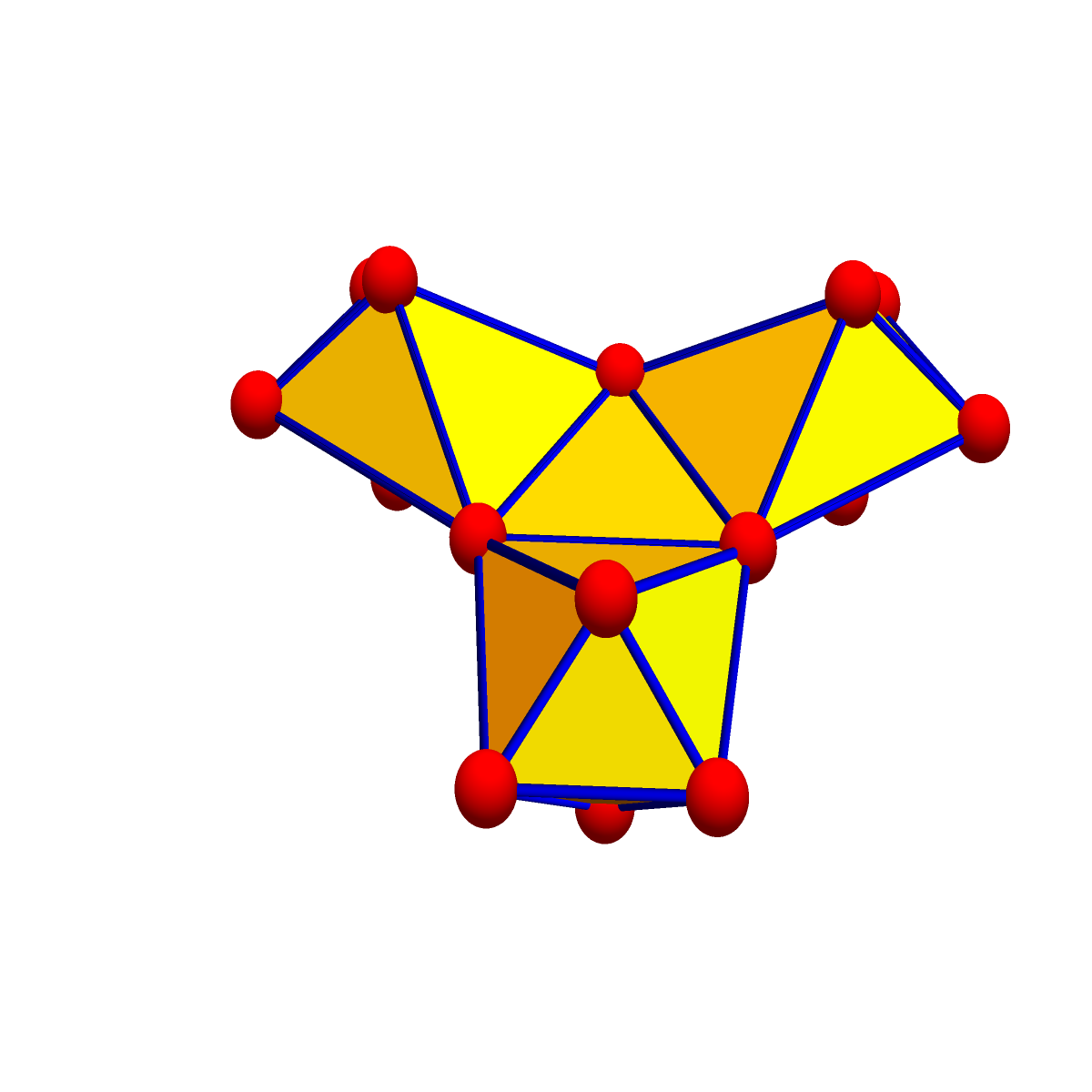
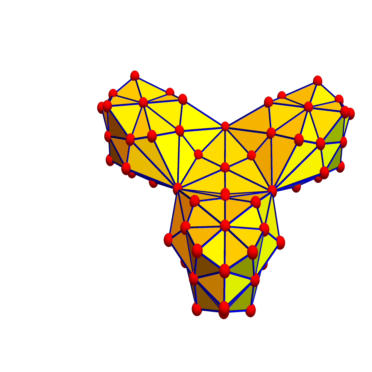
[My 25, 2017. A counter example. Take 3 octahedra. Glue them together along a triangle, not adding any further edges. This decreases the trace. Further Barycentric refinements make the trace even smaller. This example shows that even if we would ask for more refinements, the trace can become negative:
|
|
]
As we have seen above, the functional has a Gauss-Bonnet formula:
|
Gauss Bonnet: the Hydrogen trace is the sum of the curvatures K(x), where K(x) is the Euler characteristic of the unit sphere S(x). |
If the picture is right and the minima are geometric graphs, then minima have constant zero curvature. To relate with the old Gauss-Bonnet formula, in which the super curvature K(x) (-1)dim(x) is taken, then the sum is the Euler characteristic.
Dominance of positive spectrum
We also see that the positive spectrum dominates the negative spectrum. Its a bit like the Baryon asymmetry problem but of course much easier as it is a concrete problem in linear algebra. What we see is that the number of positive and negative eigenvalues of L is always very close, (even so the difference is not a combinatorial invariant). The maximal eigenvalue is larger than the absolute value of the smallest eigenvalue.
Lets define the Baryon dominance factor as  = |max(\sigma(L(G))|/|min(\sigma(L(G))|")
| Baryon dominance factor: we conjecture B(G) ≥ 2+51/2 for any complex of positive dimension. |
As for the Baryon discrepancy, the number of positive eigenvalues of L minus the number of negative eigenvalues of L, we would like to know how it grows. But we are far from that. We don’t even know yet whether there is always a negative eigenvalue! But the trace conjecture would prove it:
Trace inequality implies anti-matter
We got interested in the Hydrogen trace also because of the following corollary which deals with the negative part (anti-matter) part of the spectrum of the connection Laplacian L. One of the riddles so far was whether it is possible at all that the connection Laplacian can be positive semi-definite. As =n>0")
 = \sum_x (1-\chi(S(x)))")
| Theorem. If the Hydrogen inequality holds for G and the simplicial complex G has positive dimension, then the connection Laplacian L=L(G) has some negative eigenvalue. |
Proof. Assume L is positive semidefinite. Then also its inverse g is positive semi-definite and  \geq 0")
(i) Define the vectors Ai as  = A(i,j)")

 = -tr(H)")
")
(ii) Since ^{-1} A e_i = (1-1/(1+A)) e_i = (1-g) e_i")
 = \sum_i (e_i,(1-g) e_i) = tr(L)-tr(g) =tr(H)>0")
(iii) We now show  = -(e_i,g A_i)")
 =0")

 = (A_i, g L_i ) = (A_i, g L e_i) = (A_i,e_i)=0")
[Update of May 25: in the example with negative trace of L+ L-1 we still see negative eigenvalues.]
Existence of positive energy values
On the other hand, there is always some non-negative spectrum for L. The reason is that L is a 0-1 matrix and so has non-negative entries everywhere. A Perron-Frobenius argument gives now an eigenvector with non-negative entries. And because L is invertible, this means one of the eigenvalues has to be positive.
I currently still believe there should be an easy way to establish also that there is some negative eigenvalue of L if G has positive dimension. A simple Perron-Frobenius argument does not work yet. Sometimes it does, like if we can take vectors which are positive on even dimensional faces and negative on odd dimensional faces. Then, if the Barycentric refinement of G has constant edge degree, a Perron-Frobinus cone invariance argument (with Brouwer fixed point theorem applied to a convex subset of the sphere) shows a negative eigenvalue. In general, this argument does not bite however because the connection Laplacian does not only connect faces of different dimension parity but also connects a face with itself which has the same dimension parity. One could try to look at the spectrum of the adjacency matrix A which always has a negative eigenvalue by the above argument but this does not guarantee it for the shifted up matrix L=1+A as a priori, the negative spectrum of A could be larger than -1. So far, a simple universal argument has not appeared yet guaranteeing the existence of a negative eigenvalue. The trace inequality looks the most promising path so far.
[Update of May 23, 2017: there is some progress in describing the Hydrogen trace functional $\latex \eta(G)$. We have already seen the Gauss Bonnet formula  = \sum_{x \in G_1} \chi(S(x))")
| Gauss Bonnet II: the Hydrogen trace is the sum of the curvatures K(x), where x is a vertex of G2 with dim(x)>0 and K(x) = (-1)dim(x)+1 (dim(x)+1). |
This immediateley allows us to express the Hydrogen trace as 2 v1 – 3 v2 + 4 v2 …, where vk is the number of k-dimensional simplices in G1. So, we can express the Hydrogen trace in terms of the f-vector of G1. For 2-dimensional complexes with v vertices, e edges and f faces, we have 2 e-3f.
It gets better even: lets define the generating function  = \sum_{k=1} v_{k-1} x^{k}")
| Generating function: η(G) = h(0)-h'(-1) |
We can compare that with the Euler characteristic  = h(0)-h(-1)")
 = \sum_{k=1}^{\infty} v_{k-1} x^k")
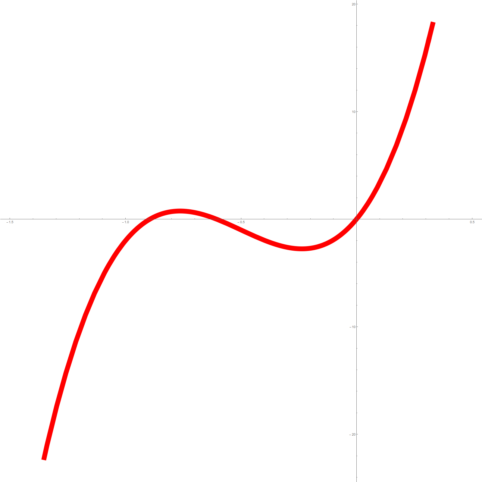
Here is an example for illustration: we see to the left the generating function of the wheel graph with 4 spikes. To the right, we see the graph of the generating function of the Octahedron graph. In the Wheel graph case, the Hydrogen trace is 8, in the Octahedron case, the Hydrogen trace is 0, the conjectured minimum. The f-vector of the Barycentric refinement of the Wheel graph is (17,40,24), the generating function is =17x+40 x^2+24 x^3")
-h'(-1)=8")
=26x+72x^2+48 x^3")
-h'(-1)=0")
In the case of the Wheel graph, the spectrum of the Hydrogen operator H is 11.1495, -8.63268, -3.65028, -3.65028, 3.65028, 3.65028, 2.64626, 2.45281, -1, -1, 1, 1, -0.821854, -0.821854, 0.821854, 0.821854, 0.384163 which adds up to tr(H)=8. In the case of the Octahedron graph, the spectrum of the hydrogen operator H is -12.1389, -5.65685, -5.65685, -5.65685, -2, -2, -2, -2, -2, -2.,0, 0, 0, 0, 0, 0, 0, 0.505882, 2, 2, 2, 2, 5.65685, 5.65685, 5.65685, 15.633 which adds up to 0.
Here are pictures of these generating functions

|
|
And here are the Hydrogen operators for the wheel and octahedron graph
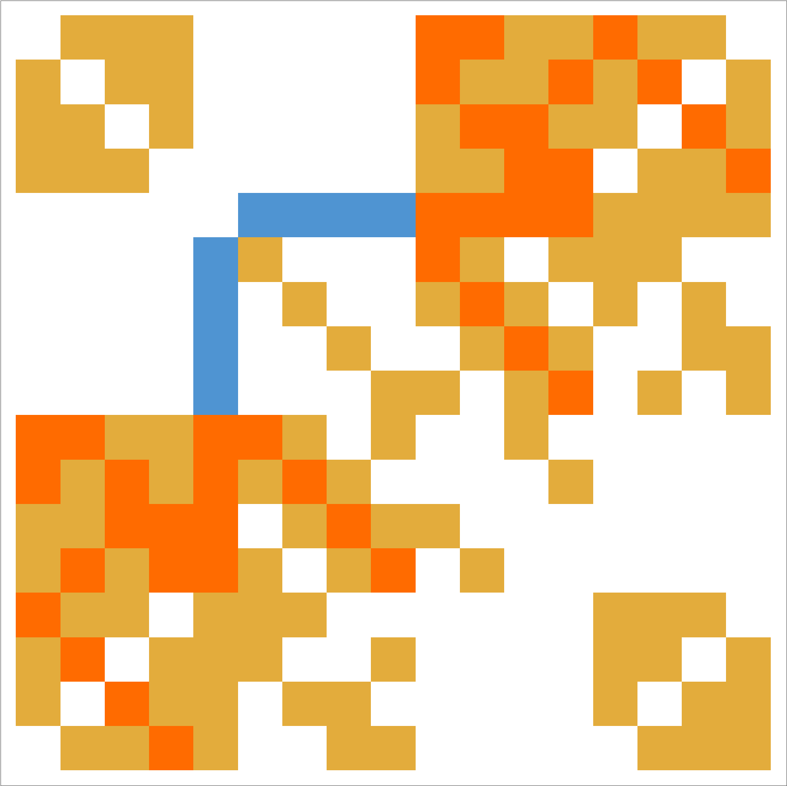
|
|
End Update]