Update of May 27, 2017: I dug out some older unpublished slides authored in 2015 and early 2016. I added something about the quantum gap and something on the quantum plane at the very end. Here is the presentation, just spoken now.
The quantum line
In one dimension, there is a natural compact metric space D on which one has a translation group which features a smallest unit. The group D of dyadic integers is the Pontyagin dual of the Pruefer group and is a natural “one-dimensional quantum space”. The real analogue is the circle, a compact topological group which is the dual of the integers and a quotient of the real numbers. The translation on D is called the adding machine. It is known in ergodic theory as the von Neumann-Kakutani system. Part of my thesis dealt with this system as it appears naturally in the context of renormalization of Jacobi matrices 


![\left[ \begin{array}{cccccccc}2&-1&0&0&0&0&0&-1\\-1&2&-1&0&0&0&0&0\\ 0&-1&2&-1&0&0&0&0\\ 0&0&-1&2&-1&0&0&0\\0&0&0&-1&2&-1&0&0\\0&0&0&0&-1&2&-1&0\\0&0&0&0&0&-1&2&-1\\-1&0&0&0&0&0&-1&2\\ \end{array} \right]](https://s0.wp.com/latex.php?latex=%5Cleft%5B+%5Cbegin%7Barray%7D%7Bcccccccc%7D2%26-1%260%260%260%260%260%26-1%5C%5C-1%262%26-1%260%260%260%260%260%5C%5C+0%26-1%262%26-1%260%260%260%260%5C%5C+0%260%26-1%262%26-1%260%260%260%5C%5C0%260%260%26-1%262%26-1%260%260%5C%5C0%260%260%260%26-1%262%26-1%260%5C%5C0%260%260%260%260%26-1%262%26-1%5C%5C-1%260%260%260%260%260%26-1%262%5C%5C+%5Cend%7Barray%7D+%5Cright%5D&bg=ffffff&fg=000000&s=0 "\left[ \begin{array}{cccccccc}2&-1&0&0&0&0&0&-1\\-1&2&-1&0&0&0&0&0\\ 0&-1&2&-1&0&0&0&0\\ 0&0&-1&2&-1&0&0&0\\0&0&0&-1&2&-1&0&0\\0&0&0&0&-1&2&-1&0\\0&0&0&0&0&-1&2&-1\\-1&0&0&0&0&0&-1&2\\ \end{array} \right]")
The matrix 4 B – B.B decomposes into two copies of the Kirchhoff matrix of C4:
![\left[\begin{array}{cccccccc} 2&0&-1&0&0&0&-1&0\\0&2&0&-1&0&0&0&-1\\-1&0&2&0&-1&0&0&0\\0&-1&0&2&0&-1&0&0\\0&0&-1&0&2&0&-1&0\\ 0&0&0&-1&0&2&0&-1\\-1&0&0&0&-1&0&2&0\\0&-1&0&0&0&-1&0&2\\\end{array}\right]](https://s0.wp.com/latex.php?latex=%5Cleft%5B%5Cbegin%7Barray%7D%7Bcccccccc%7D+2%260%26-1%260%260%260%26-1%260%5C%5C0%262%260%26-1%260%260%260%26-1%5C%5C-1%260%262%260%26-1%260%260%260%5C%5C0%26-1%260%262%260%26-1%260%260%5C%5C0%260%26-1%260%262%260%26-1%260%5C%5C+0%260%260%26-1%260%262%260%26-1%5C%5C-1%260%260%260%26-1%260%262%260%5C%5C0%26-1%260%260%260%26-1%260%262%5C%5C%5Cend%7Barray%7D%5Cright%5D&bg=ffffff&fg=000000&s=0 "\left[\begin{array}{cccccccc} 2&0&-1&0&0&0&-1&0\\0&2&0&-1&0&0&0&-1\\-1&0&2&0&-1&0&0&0\\0&-1&0&2&0&-1&0&0\\0&0&-1&0&2&0&-1&0\\ 0&0&0&-1&0&2&0&-1\\-1&0&0&0&-1&0&2&0\\0&-1&0&0&0&-1&0&2\\\end{array}\right]")
Indeed, the Julia set of the quadratic map
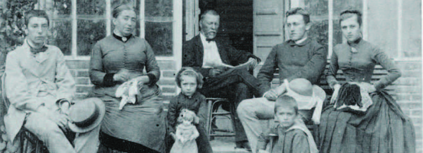
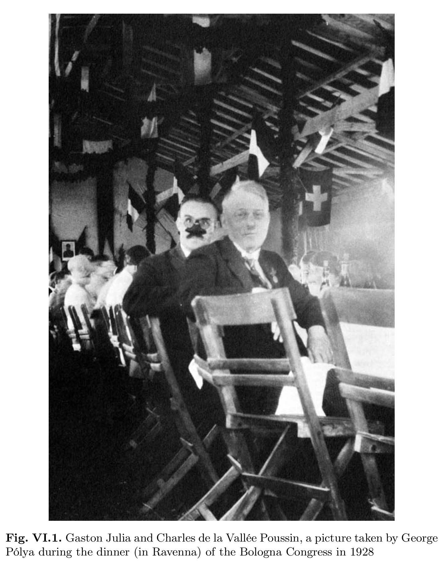
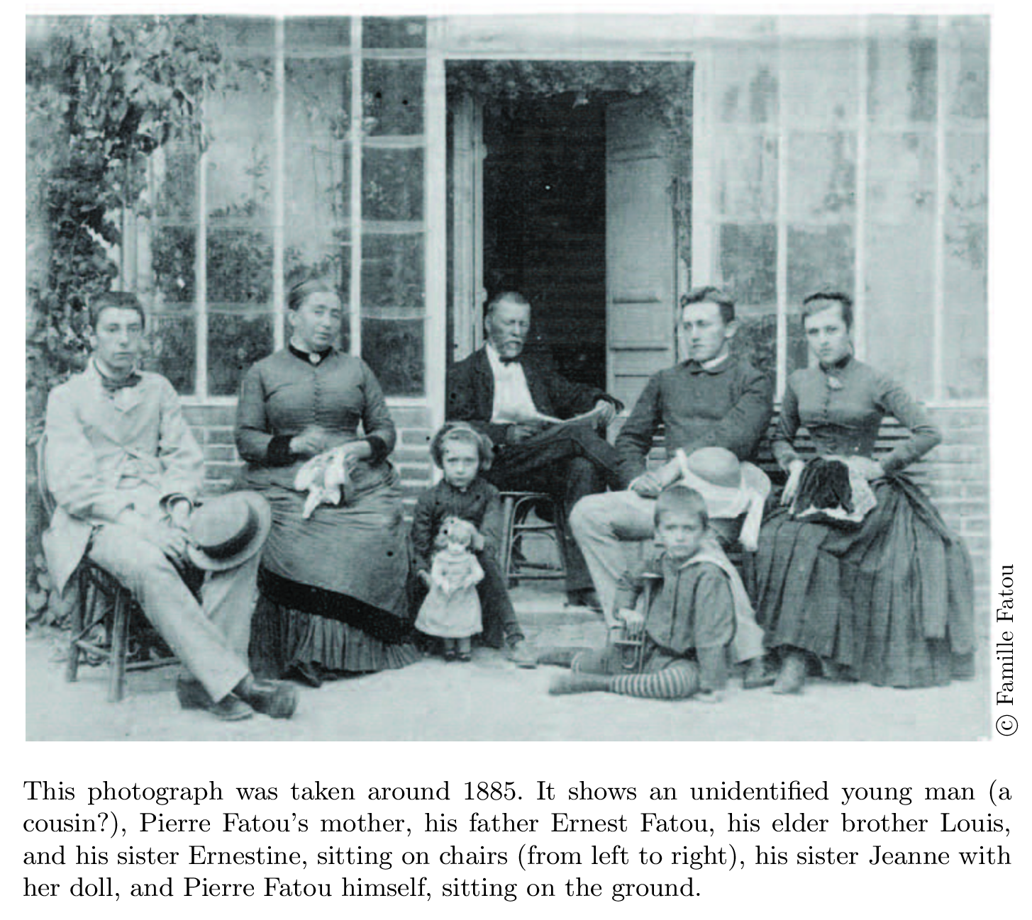
 = z(4-z)") is the interval [0,4]. This picture gives the density of states in the Barycentric limit of a one dimensional simplicial complex. Apropos: here are two unusual photos of Julia and Fatou. They are from the book of Michele Audin “Fatou, Julia, Montel”, Springer Lecture Notes in Mathematics 2014. Click on the picture to see it large:
is the interval [0,4]. This picture gives the density of states in the Barycentric limit of a one dimensional simplicial complex. Apropos: here are two unusual photos of Julia and Fatou. They are from the book of Michele Audin “Fatou, Julia, Montel”, Springer Lecture Notes in Mathematics 2014. Click on the picture to see it large:
|
|
Two dimensional quantum space
We tried to get a grip on higher dimensional versions here [PDF]. The following construction was done in thesis (page 250) We proved that the renormalization map for Z^d systems has a unique fixed point. Lets look at the construction in two dimensions:
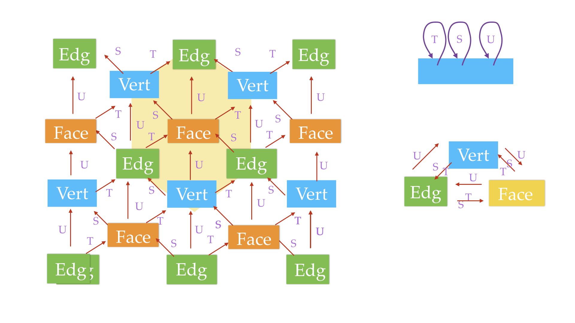
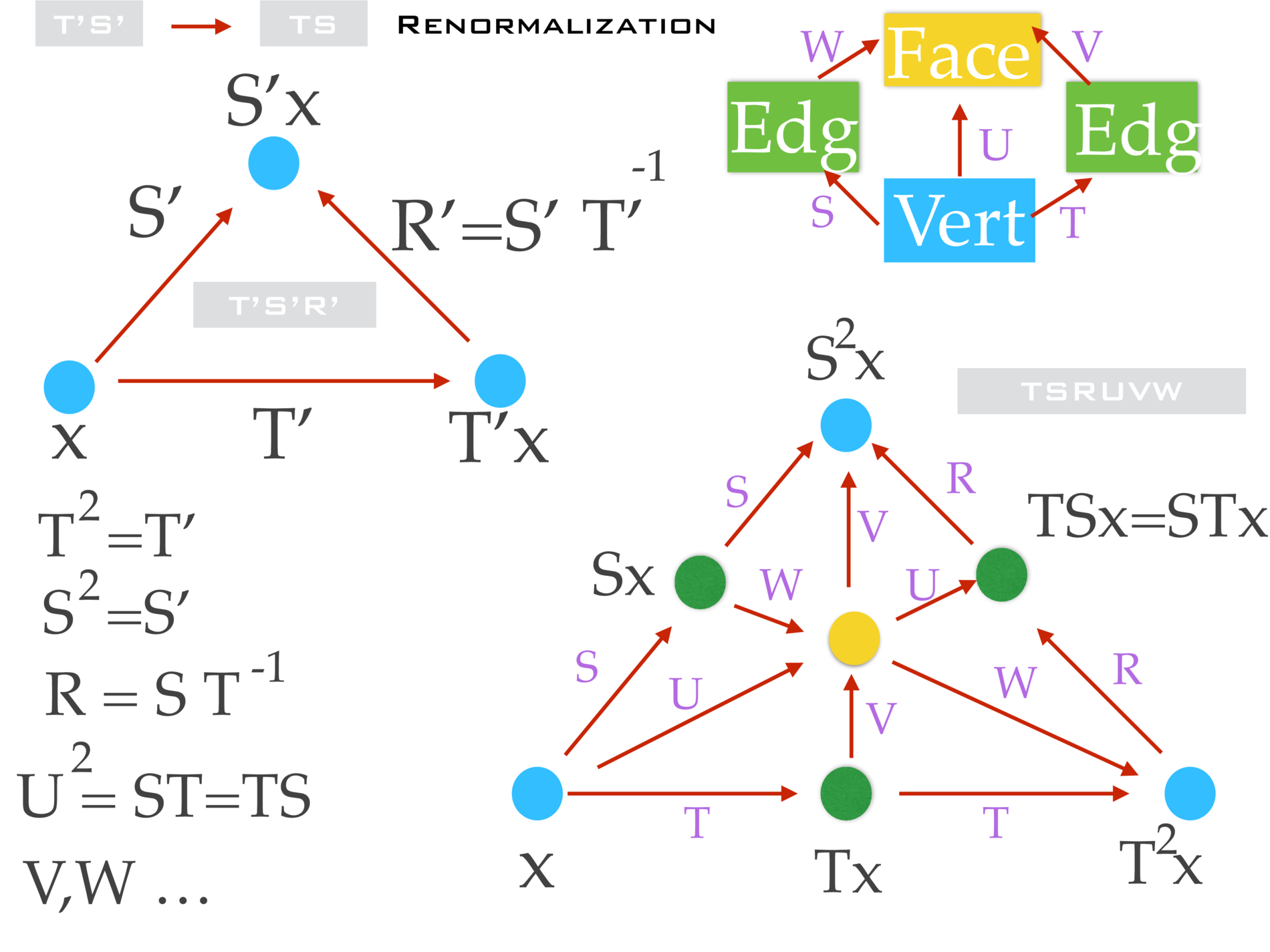
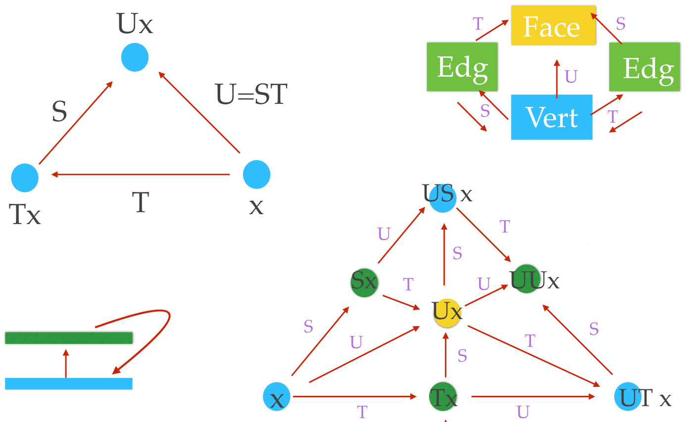
In October 2015, we started to investigate the Barycentric limit in the 2 dimensional case. It is a renormalizaation story on pairs (T,S) of commuting measure preserving transformations. This generalizes the von Neumann-Kakutani case. First make integral extensions T_1^2=T, S_1^2=S, U^2 = ST = TS.
Definition. Let T,S be a pair of commuting automorphisms (measure preserving invertible maps) of a Lebesgue space, (a standard probability space) X. Define a new system by taking a union of 4 copies of X1,X2,X3,X4.
On X1, define T1: X1 -> X2     x -> Tx
On X1, define S1: X1 -> X3     x -> Sx
On X2, define T1: X2 -> X1     x -> x
On X2, define S1: X2 -> X4     x -> Sx
On X3, define T1: X3 -> X1     x -> x
On X3, define S1: X3 -> X4     x -> Tx
On X4, define T1: X4 -> X3     x -> Sx
On X4, define T2: X4 -> X2     x -> Tx
Now, 


 \to (X1,T1,S1)")
,(U,V)) = m( \{ x \; |\; T(x) \neq U(x) or S(x) \neq V(x) \}")

A martingale idea
But that produces a mess of transformations. It would be nicer to have only two transformations and look at their orbits. Depending on the sigma-alrebra used, we would get the individual Barycentric refinements. This is kind of a Martingale idea: play with the 
Here is an other doodle. It might be better to renormalize the Z2 action with tripling the probability space each time: