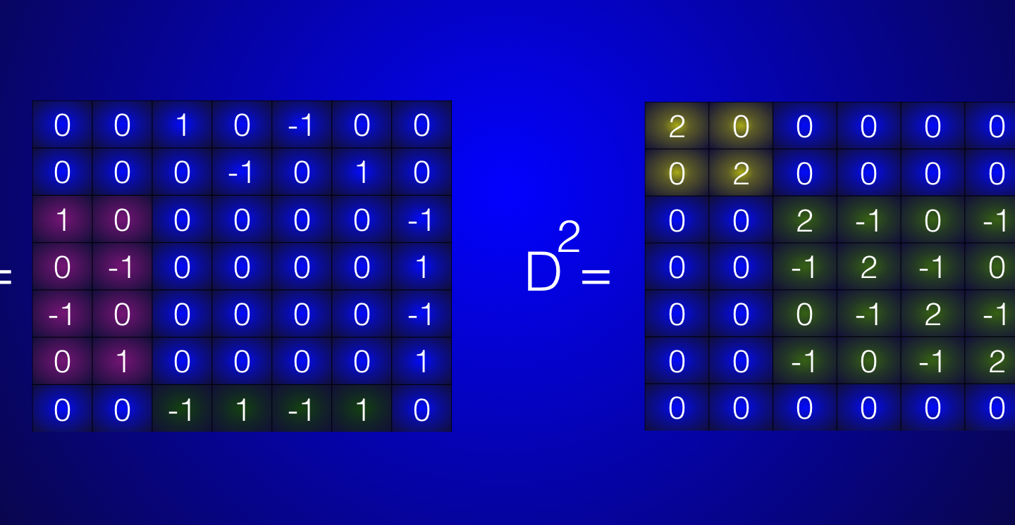
In our second linear algebra midterm of math 21b, the quadratic interaction cohomology was the topic of problem 7. There are some remarks in the solutions already. In that problem 7 we looked at a matrix $H$ which his the quadratic Hodge Laplacian” of the complete graph of two elements. When doing interaction calculus, not the individual components of space but the individual pairs of space components are of interest. In this particular case when “space” consists of two points $a,b$ only connected with a connection link $e$ we have the simplest positive dimensional “world” one can build. (In the zero dimensional case, there are only the self interactions of points with themselves and nothing interesting happens). Here is the matrix
$$ H = \left[
\begin{array}{clccccl}
2 & 0 |& 0 & 0 & 0 & 0 &| 0 \\
0 & 2 |& 0 & 0 & 0 & 0 &| 0 \\ \hline
0 & 0 |& 2 & -1 & 0 & -1 &| 0 \\
0 & 0 |& -1 & 2 & -1 & 0 &| 0 \\
0 & 0 |& 0 & -1 & 2 & -1 &| 0 \\
0 & 0 |& -1 & 0 & -1 & 2 &| 0 \\ \hline
0 & 0 |& 0 & 0 & 0 & 0 &| 4 \\
\end{array}
\right] \; $$
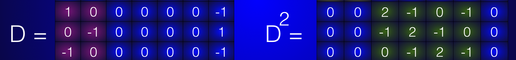
It satisfies $H=D^2$ with
$$ D = \left[
\begin{array}{ccccccc}
0 & 0 & 1 & 0 & -1 & 0 & 0 \\
0 & 0 & 0 & -1 & 0 & 1 & 0 \\
1 & 0 & 0 & 0 & 0 & 0 & -1 \\
0 & -1 & 0 & 0 & 0 & 0 & 1 \\
-1 & 0 & 0 & 0 & 0 & 0 & -1 \\
0 & 1 & 0 & 0 & 0 & 0 & 1 \\
0 & 0 & -1 & 1 & -1 & 1 & 0 \\
\end{array}
\right] \; . $$
The $D$ incorporates the exterior derivatives $d_0: \Lambda^0 \to \Lambda^1$ and $d_1: \Lambda^1 \to \Lambda^2$. We have $d_0=\left[ \begin{array}{cc} 1 & 0 \\ 0 & -1 \\ -1 & 0 \\ 0 & 1 \end{array} \right]$ and $d_1=\left[ \begin{array}{cccc} -1 & 1 & -1 & 1 \end{array} \right]$. The derivative $d_0$ which maps $0$-forms to $1$-forms is kind of a gradient, while $d_1$ which maps $1$-forms to $2$-forms is a kind of curl. It is a bit strange here as we have a one-dimensional space only, but the interaction forms dealing with the self-interaction of the one-dimensional part of space is a 2-form here.
The interaction components in $K_2$ are given by the 7 possible pairs $(a,a),(b,b),(a,e),(b,e),(e,a),(e,b),(e,e)$ of intersecting components of zero dimensional parts $a,b$ and one dimensional part $e$. This leads to the $7 \times 7$ matrix above). One can now do everything of the usual calculus and physics also on this new connection calculus. For example, in quantum mechanics, a Laplacian models the kinetic energy of a particle. It completely describes the motion of a single non-interacting particle. The equation $u_{tt} = – H u$ is the wave equation which describes the motion of a particle in that world. It has the solution $\cos(D t) u(0) + \sin(D t) D^{-1} u'(0)$ (as $D$ is not invertible, the inverse is taken on the eigenspaces of non-zero eigenvalues, this is called the “pseudo inverse”. To check the identity, just differentiate twice. $d^2/dt^2 \cos(Dt) = -D^2 \cos(Dt)=-H \cos(Dt)$). If you define the complex vector $\psi(t) = u(t) + i D^{-1} u'(t)$, then because $e^{i D t} = \cos(D t) + i \sin(D t)$ (Euler), the solution of the wave equation can also be written as $e^{-i Dt} \psi(0)$. In other words, the solution satisfies the Schr\”odinger equation $i \psi'(t) = D \psi(t)$. Now this works on any network. The point of the factorization $D^2=H$ is that it allows to give explicit solutions of the wave equation on a network for example. It is quite easy to to write down the operator $D$ for any “world”. The factorization for the usual Laplacian $d^2/dx^2 + d^2/dy^2 + d^2/dz^2 = {\rm div(grad)}$ had first been done by Paul Dirac (who was motivated by physics too but also liked mathematical beauty and symmetry). It required Dirac matrices. In the discrete, we don’t need that gymnastics. Things are much easier. The fact that physics on finite spaces is orders of magnitudes less technical than the physics in the continuum prompted physicists and philosophers to suggest space is actually discrete. Already Gottfried Leibniz started such thoughts. But it still remains just speculation. What counts in physics are affinities with real experiments: predictions of quantitative nature about physical processes which can be measured and verified. Until then, it is mathematics – or what is almost the same – poetry.
We have given in part b) the information that if $\lambda$ is an eigenvalue of $D$, then $-\lambda$ is an eigenvalue too. This is a consequence of what one calls {\bf super symmetry} (in a purely mathematical sense, unlike in physics, mathematical super symmetry is always present. Physicists love symmetry so much that they believed for a long time that a stronger version holds fundamentally and that every particle has a super partner. Experiments at the Large Hadron Collider at CERN in the last decade have severely supressed this dream even so many still have hope.) In mathematics, there is no problem. It is a mathematical fact that it always appears and here is the proof: we can write $D = \left[ \begin{array}{cc} 0 & A \\ A & 0 \end{array} \right]$ with block matrices $A$. Now define the diagonal matrix $P=\left[ \begin{array}{cc} I & 0 \\ 0 & -I \end{array} \right]$ where $I$ is the identity matrix. The simplest notion of mathematical super-symmetry (as coined and used by Ed Witten in purely mathematical frame works) are the matrix relations $L=D^2, P^2=1, D P + P D = 0$. You can check that these symmetries hold. Now, if $D v = \lambda v$, then $P D P v = – D P P v = – D v = – \lambda v$. We see that $P v$ is an other eigenvector, but with an eigenvalue $-\lambda$. The “particle” belonging to the energy $-\lambda$ is the “anti-particle” to the particle belonging to the energy $\lambda$. This zero-dimensional version of super symmetry is actually present in physics as we have seen anti-particles (Dirac got the Nobel prize in 1933 jointly with Erwin Schroedinger for that). Physicists have not seen super particles yet in particle accelerations. Maybe they don’t exist.
This computation actually computed the Betti vector $(b_0,b_1,b_2)=(0,1,0)$ in a {\bf “cohomology”} defined by this one-dimensional network. his sounds fancy but it is just an impressive name for the kernels of some matrices. The number $b_0$ is the nullity of the first block, the number $b_1$ is the nullity of the second block, the number $b_2$ is the nullity of the third block. The number $b_0-b_1+b_2$ is the Wu characteristic of the network. It is defined as $\sum_{x \sim y} \omega(x) \omega(y)$, where $\omega(x)=(-1)^{dim(x)}$ and $x \sim y$ means that the two components are connected. In the case of the network under consideration, we have $7$ summands and since $\omega(a)=\omega(b)=1$ and $\omega(e)=-1$, we have a sum of $7$ terms $\omega(a) \omega(a) + … + \omega(e) \omega(e)=-1$. The fact that the alternating sum of the Betti numbers (an algebraically defined notion) is the same than the combinatorially computed notion is a higher order version of the Euler-Poincar\’e theorem (which does the same in traditional calculus). The fact that the Betti numbers can be expressed as the nullity of the block matrices appearing in $H$.