In my paper “Manifolds from Partitions”, I stated that that the case of empty graphs can not occur, but did not prove it. It is indeed not true. Here is an update [PDF] with an additional section. It is very rare although that a surjective map produces still an empty surface. Last week, I made some experiments with all surjective maps 


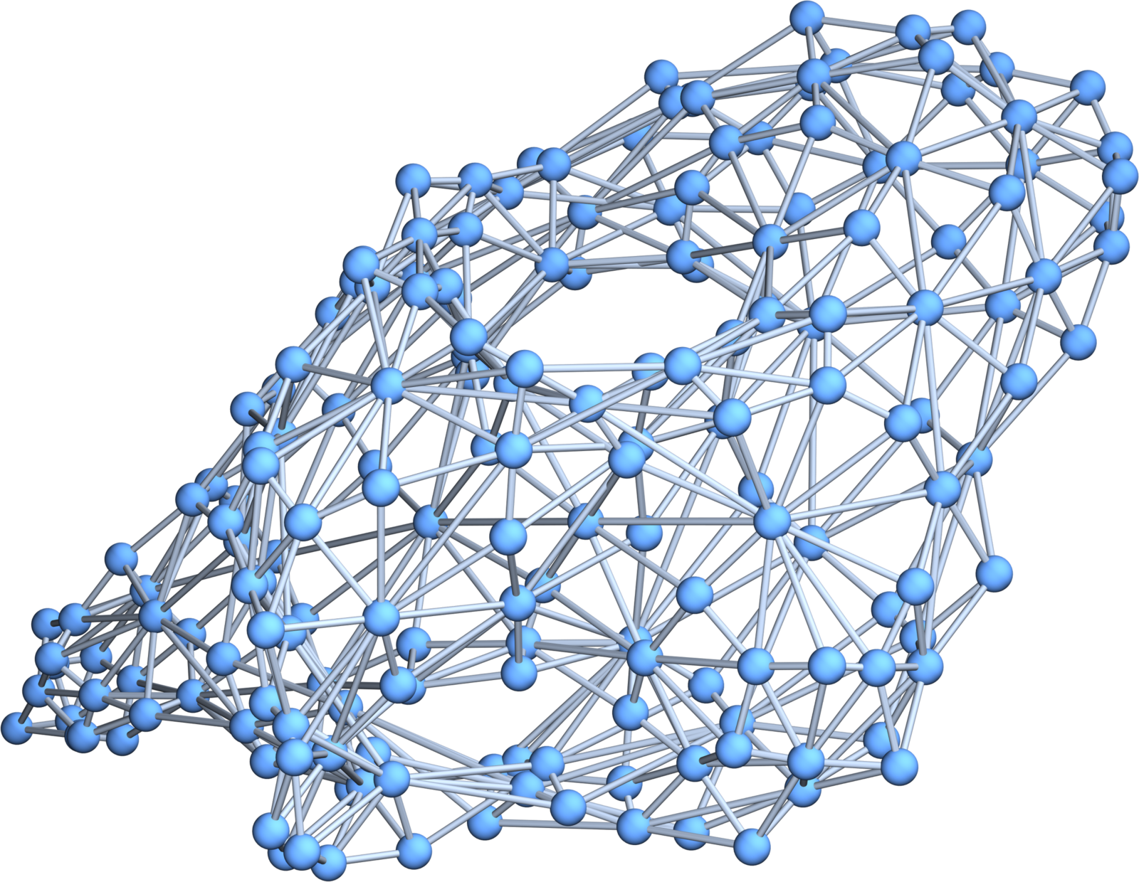
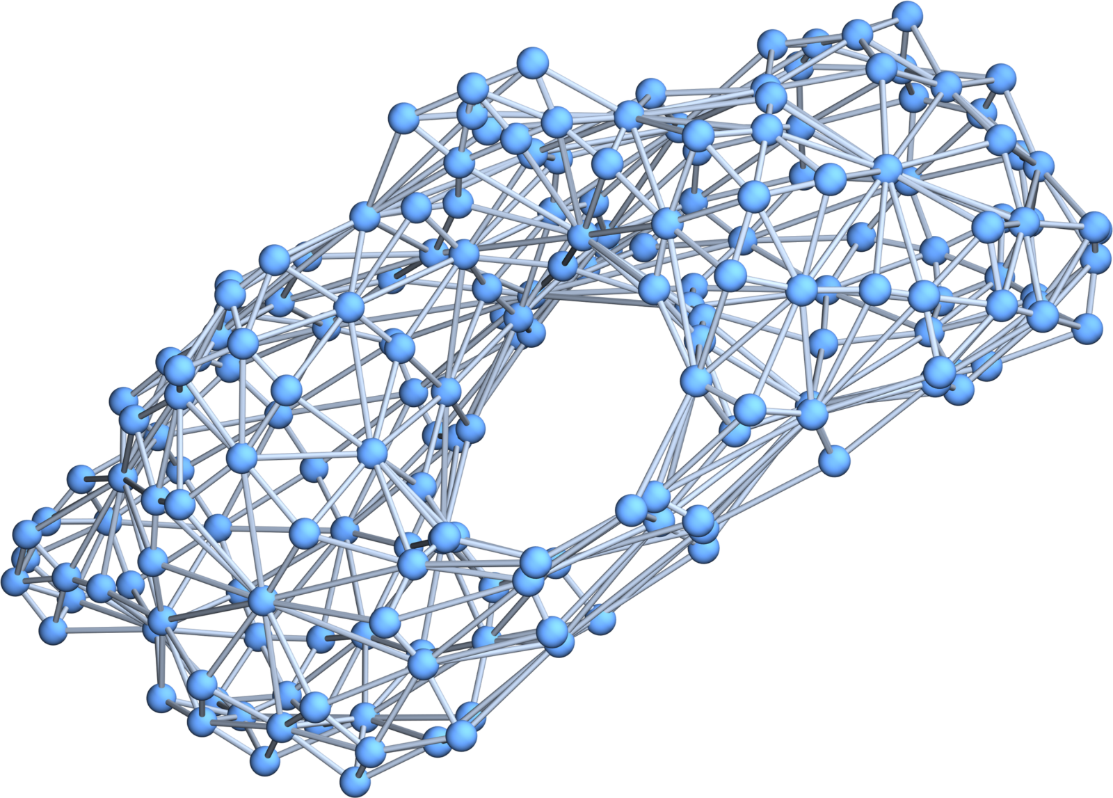
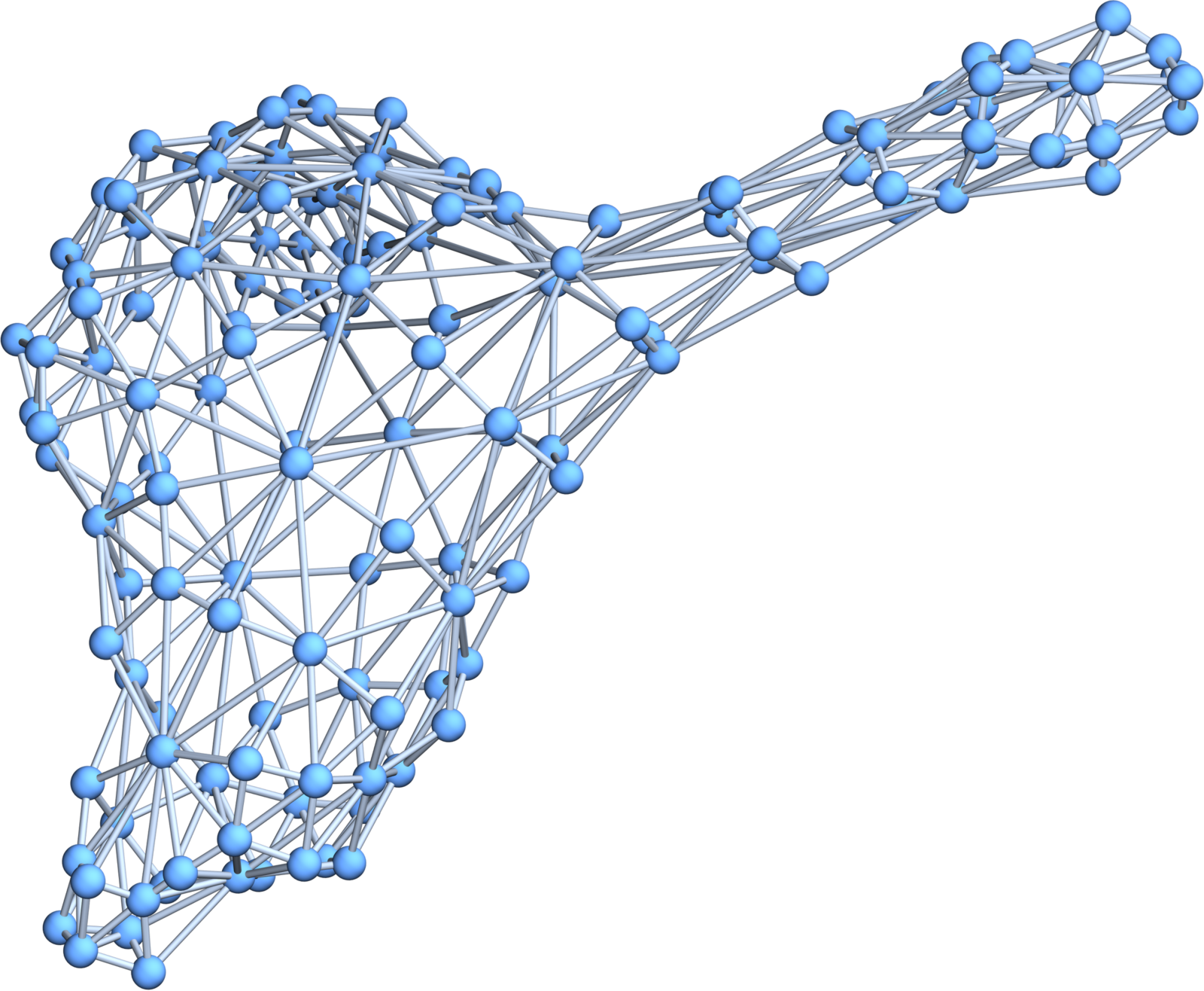
Here is the code which was used to compute: (also included in the update). It was submitted also on the ArXiv so that it could be grabbed there from the LaTeX source of the paper. The first few lines use the “5 lines are enough for cohomology” https://www.quantumcalculus.org/the-5-lines-of-cohomology/ . I used that cohomology code essentially verbatim and did not bother shifting the Betti vectors. As we have a priori delta sets there are always some zeros before as we do not have simplicial complexes but delta sets which are shifted simplicial complexes in the sense that just the dimension attached to each class of sets is shifted. If we compute these “level surfaces” or codimension k surfaces in the host manifold G, the sets are a priori open sets in the Alexandrov topology of the complex. They are so delta-sets, my now favorite discrete structure as it is a topos. But they are manifolds if one attaches the right dimension type. When computing the cohomology of a surface obtained by taking a map from G to K3 for example, we get a codimension 2 surface. It is made up of all the simplices in the complex for which the image contains the triangle K3. Of course, the “zero dimensional points” are the 2 dimensional simplices in G. These are the points of the surface, the 4-cliques are the edges and the 5-cliques are the triangles in the surface. This is a nice example where delta sets appear naturally. I should also reiterated again that delta sets are more general than simplicial sets. Simplicial sets have more structure and so form a special class of delta sets. It is the topos of delta sets which we should focus on. (The code below just also includes an example where a random surface is picked. In the paper, I include the code to generate “All surfaces”. This is a task which only can be done for very small host manifolds G with like with 11 points, where 3^11 is 177147. We can still compute all the cohomologies of 177147 codimension 2-manifolds in a reasonable time. The example given below uses the Hopf 4-manifold S2xS2 (which is one of my favorite 4 manifolds because there are so many open questions about it) I have spent a considerable amount of time in my llife with the Hopf conjectures in differential geometry. It is still open problem for example, whether S2xS2 can carry a metric of positive curvature. Using discrete manifolds is the way to try out experimentally. Here is an entry in this blog about it from 2020, when I spent a few months intensively with the conjectures. I was looking then at curvature as the expectation of Poincare-Hopf indices and searched also with curvatures satisfying Gauss-Bonnet-Chern which are positive if all the sectional curvatures are positive. At one point, I thought to have found a candidate of such a curvature. This is much more flexible than the rigid Gauss-Bonnet-Chern integrand in the continuum but of course, it can also be done in the continuum. Just fix a probability measure on the set of Morse functions and you have a curvature satisfying Gauss-Bonnet. A global curvature on a manifold should definitely satisfy Gauss-Bonnet or be of interest in other ways, like the scalar curvature, which does not satisfy Gauss-Bonnet but when integrated produces the Hilbert action in general relativity. Now, of course, S2xS2 has Euler characteristic 2×2 = 4 so that there are lots of points where the Gauss-Bonnet-Chern curvature (Euler integrand, a Pfaffian of the Riemann curvature tensor) and so also some sectional curvatures are positive. The open problem is to find a metric so that all sectional curvatures are positive. Using probability measures to define what “sectional curvature” is also allows to be more flexible. The product metric in the continuum always has some flat planes: pick a vector in the first S2 and a vector in the second sphere S2. These two vectors span a plane which defines a 2-plane in the tangent space of a point for which the sectional curvature is zero. By the way, if you enter the code below and enter Betti[S2xS2] you get the Betti vector (1,0,2,0,1) which is the convolution of (1,0,1) and (1,0,1), the Betti vectors of the factors, as it should be. The Poincare polynomial 
^2 = 1+2t^2+t^4")
Generate[A_]:=If[A=={},{},Sort[Delete[Union[Sort[Flatten[Map[Subsets,A],1]]],1]]];
Whitney[s_]:=Generate[FindClique[s,Infinity,All]];L=Length; Ver[X_]:=Union[Flatten[X]];
sig[x_]:=Signature[x]; nu[A_]:=If[A=={},0,L[NullSpace[A]]];
F[G_]:=Module[{l=Map[L,G]},If[G=={},{},Table[Sum[If[l[[j]]==k,1,0],{j,L[l]}],{k,Max[l]}]]];
sig[x_,y_]:=If[SubsetQ[x,y]&&(L[x]==L[y]+1),sig[Prepend[y,Complement[x,y][[1]]]]*sig[x],0];
Dirac[G_]:=Module[{f=F[G],b,d,n=L[G]},b=Prepend[Table[Sum[f[[l]],{l,k}],{k,L[f]}],0];
d=Table[sig[G[[i]],G[[j]]],{i,n},{j,n}]; {d+Transpose[d],b}];
Beltrami[G_]:= Module[{B=Dirac[G][[1]]},B.B];
Hodge[G_]:=Module[{Q,b,H},{Q,b}=Dirac[G];H=Q.Q;Table[Table[H[[b[[k]]+i,b[[k]]+j]],
{i,b[[k+1]]-b[[k]]},{j,b[[k+1]]-b[[k]]}],{k,L[b]-1}]];
Betti[s_]:=Module[{G},If[GraphQ[s],G=Whitney[s],G=s];Map[nu,Hodge[G]]];
Facets[G_]:=Select[G,(L[#]==Max[Map[L,G]]) &]; Poly[X_]:=PolyhedronData[X,"Skeleton"];
AbstractSurface[G_,f_,A_]:=Select[G,(Sum[If[SubsetQ[#/.f,A[[l]]],1,0],{l,L[A]}]>0)&];
Z[n_]:=Partition[Range[n],1]; ZeroJoin[a_]:=If[L[a]==1,Z[a[[1]]],Whitney[CompleteGraph[a]]];
CJoin[G_,H_]:=Union[G,H+Max[G]+1,Map[Flatten,Map[Union,Flatten[Tuples[{G,H+Max[G]+1}],0]]]];
RFunction[G_,P_]:=Module[{},R[x_]:=x->RandomChoice[Range[L[Ver[P]]]];Map[R,Ver[G]]];
S2xS2=Generate[{{1,2,3,4,6},{1,2,3,4,7},{1,2,3,6,9},{1,2,3,7,9},{1,2,4,5,8},{1,2,4,5,9},
{1,2,4,6,8},{1,2,4,7,9},{1,2,5,6,8},{1,2,5,6,9},{1,3,4,6,7},{1,3,5,6,7},{1,3,5,6,9},
{1,3,5,7,10},{1,3,5,9,11},{1,3,5,10,11},{1,3,7,9,10},{1,3,9,10,11},{1,4,5,8,10},
{1,4,5,9,11},{1,4,5,10,11},{1,4,6,7,11},{1,4,6,8,10},{1,4,6,10,11},{1,4,7,9,11},
{1,5,6,7,8},{1,5,7,8,10},{1,6,7,8,11},{1,6,8,10,11},{1,7,8,10,11},{1,7,9,10,11},
{2,3,4,6,8},{2,3,4,7,8},{2,3,5,7,10},{2,3,5,7,11},{2,3,5,10,11},{2,3,6,8,10},{2,3,6,9,10},
{2,3,7,8,11},{2,3,7,9,10},{2,3,8,10,11},{2,4,5,8,9},{2,4,7,8,9},{2,5,6,8,11},{2,5,6,9,10},
{2,5,6,10,11},{2,5,7,8,9},{2,5,7,8,11},{2,5,7,9,10},{2,6,8,10,11},{3,4,6,7,11},{3,4,6,8,10},
{3,4,6,9,10},{3,4,6,9,11},{3,4,7,8,11},{3,4,8,9,10},{3,4,8,9,11},{3,5,6,7,11},{3,5,6,9,11},
{3,8,9,10,11},{4,5,6,9,10},{4,5,6,9,11},{4,5,6,10,11},{4,5,8,9,10},{4,7,8,9,11},{5,6,7,8,11},
{5,7,8,9,10},{7,8,9,10,11}}];
P=ZeroJoin[{1,1,1}]; H=AbstractSurface[S2xS2,RFunction[S2xS2,P],Facets[P]];
Print[Betti[H]];
ToGraph[G_]:=UndirectedGraph[n=L[G];Graph[Range[n],
Select[Flatten[Table[k->l,{k,n},{l,k+1,n}],1],(SubsetQ[G[[#[[2]]]],G[[#[[1]]]]])&]]];
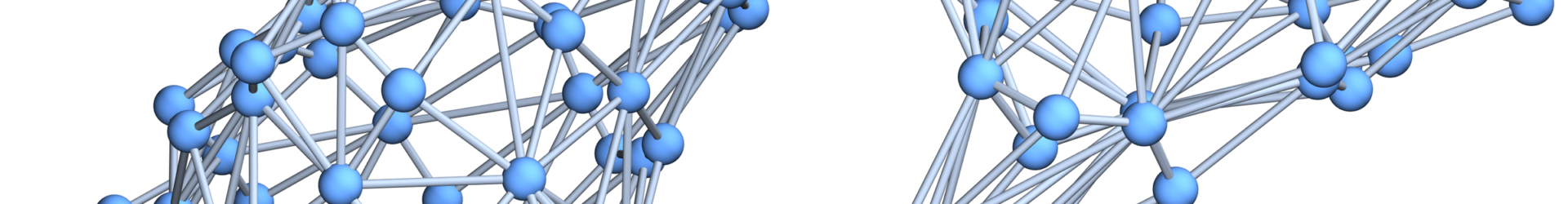
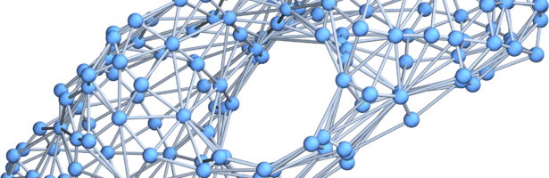
GraphPlot3D[ToGraph[H]]
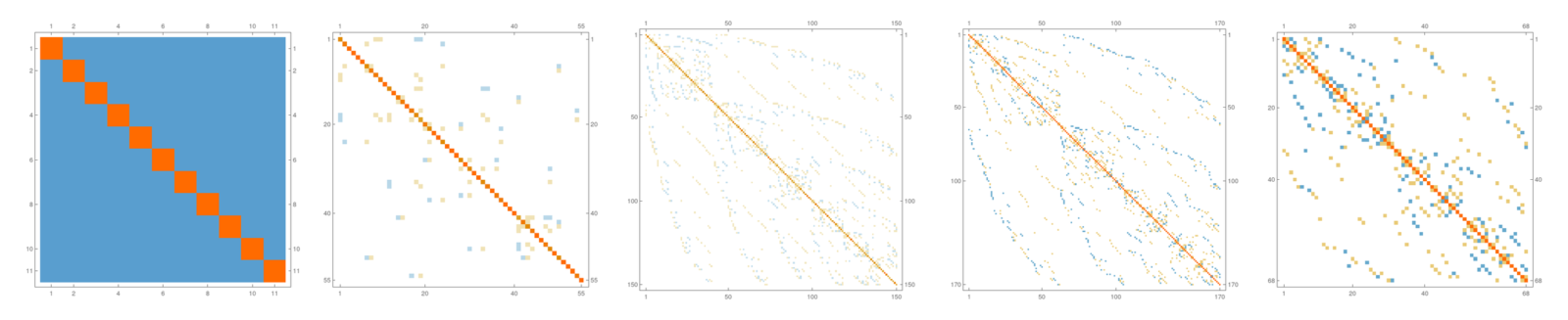
MatrixPlot[Beltrami[S2xS2]] (* The Hodge Matrix of the 4-manifold S2xS2 *)
Map[MatrixPlot, Hodge[S2xS2]] (* The 5 individual blocks of that matrix *)
Map[NullSpace, Hodge[S2xS2]] (* Explicit basis for the cohomology groups *)