A quaternion valued elliptic complex

This blog entry delivers an other example of an elliptic complex which can be used in discrete Atiyah-Singer or Atiyah-Bott type setups as examples. We had seen that when deforming an elliptic complex with an integrable Lax deformation, we get complex elliptic complexes. We had wondered in that blog entry whether a complex can lead to quaternion-valued fields. The discussion which follows here is all in a setting where the underlying geometry is a finite abstract simplicial complex. It almost verbatim would apply also to elliptic complexes over Riemannian manifolds.

Quantum dynamics

Quantum mechanics studies the unitary evolution , where D is selfadjoint operator on a Hilbert space. Given a state encoding the initial situation, one gets the future so that solves the wave equation with initial condition and initial velocity . The analogy is perfect if is a Laplacian. Since the Schrödinger equation for a complex wave is equivalent to the wave equation for a real valued wave, quantum mechanics is also called “wave mechanics”. It is quite amazing that on a fundamental level, the mathematics of quantum mechanics is simpler than classical mechanics, where one has non-linear dynamical systems. It is also remarkable also that on a fundamental level, complex valued fields appear naturally. The unitary dynamics is at the core of quantum mechanics. When discussing the system itself, one can avoid discussing the role of measurements. There are still many mathematical problems: like the relation between spectral properties of D and the dynamical transport properties of the wave. Even before that there is the problem to determine the nature of the spectrum for concrete Hamiltonians in the continuum. In applications like chemistry, one wants to make quantitative predictions about chemical properties of matter, in cryptological applications one wants to use the system secure message transmission and in computer science one aims to use the dynamics for making computations. Still, the underlying dynamical system could not be simpler: the trajectory of simple path in an unitary group. But this evolution is not the most general one as there is a symmetry present. But any unitary conjugation of D produces a system which is equivalent. We just watch it from a different point of view. Principles of relativity have historically been very successful. So much that they appear to be a cliché (but that should note make them less important). It is also entrenched in quantum mechanics: unitarily equivalent operators produce equivalent physics as chosing a particular coordinate system is just chosing a particular basis in the Hilbert space.

Quaternion valued waves

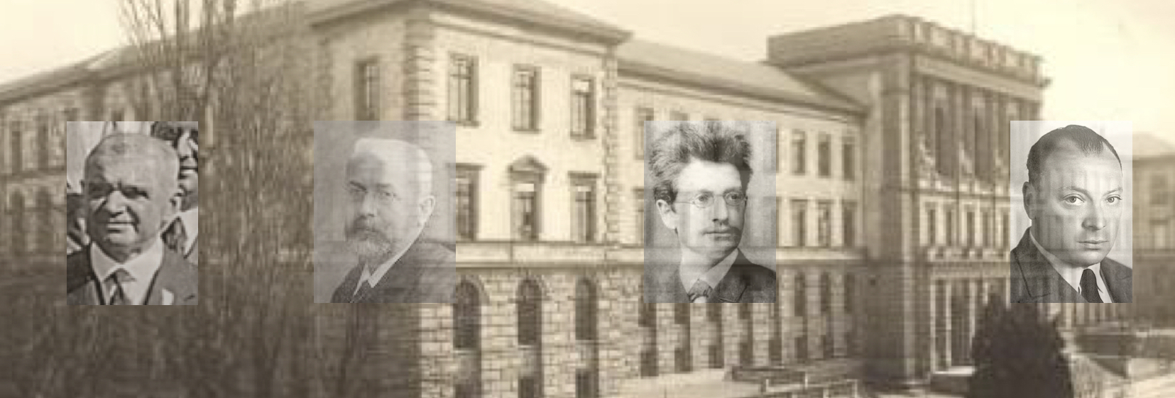
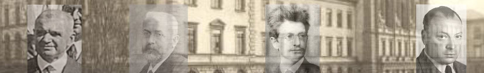
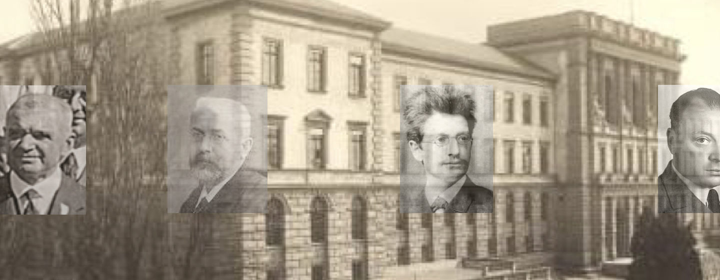
By results of Hurwitz and Frobenius, the list of associative complete division algebras contains only two elements: the complex numbers and the quaternions. This is related to the fact that spheres in Euclidean spaces Rⁿ are connected Lie groups only if n=2 or n=4. Both completeness as well as associativity are important in a dynamical quantum frame work. This excludes the other two division algebras: the real line is not complete and the octonion algebra is not associative. As complex-valued field naturally enter quantum dynamics, it is natural to ask whether quaternion-valued fields are relevant. It was Rudolf Fueter, a student of David Hilbert, who has investigated the Dirac equation for quaternion valued fields and saw it as a Cauchy-Riemann type equation. All three, Adolf Hurwitz, Ferdinand Frobenius and Rudolf Fueter were Zurich-based for part of their careers.

Do quaternion-valued waves appear naturally in quantum dynamics? If one would insist also on commutativity, the complex plane would be the unique division algebra, but in a quantum frame work, we really do not want to insist on commutativity. So, we have to look at quaternion-valued fields too. But they have to appear naturally in the sense that we don’t want to place the structure in artificially. It should emerged by itself! Now there appears a superficial difficulty with quaternion-valued matrices like that one can not define naturally a determinant for such matrices. But this is no problem as we can look at complex matrices as real matrices, we can also look at quaternion-valued matrices as complex-valued matrices. This is known as under the name of Cayley-Dickson construction and allows us to deal with complex matrices.

From geometry to dynamics

Given a geometric space like a simplicial complex or CW complex G or a ring element generated by such objects, there are natural incidence matrices d and so a Dirac operator D and a Laplacian L=D². More generally we have elliptic complexes defined over G. What matters is the spectrum of D as well as how the eigenfunctions are linked to geometry. One way how D links to geometry is that D determines the geometry: it is possible to measure distances on all dimension level using the Connes formula. Given two simplices x,y, their distance is the supremum over all , where f runs over all functions satisfying . This formula links the algebra with distances in the geometry. Now, if we let the operator evolve freely in its symmetry group, we can get complex valued or even quaternion valued operators. What quantum dynamics should we chose? Given any unitary path V(t) we can look at D(t) = V(t)^* D(0) V(t). Now taking V(t)=exp(i tD) or any V(t)=exp(i t f(D)) does not work as V(t) commutes with D so that there is no motion. So, if we want to move, the deformation of the operator D has to be done with something not obtained directly from the functional calculus of D. What works is a Lax deformation, or equivalently introducing a symplectic structure. A functional H(L)=tr(h(L)) can be seen as a Hamiltonian function. Its gradient is h'(L). The analogue of a symplectic matrix J changing the classically the gradient flow on the cotangent bundle into a Hamiltonian system is replacing d/dt L = h'(L) with d/dt L = [B(L),h'(L)].

A tumbling rock analogy

As a motivation for the following lets look at the analogy of a rock moving through space without the influence of any external force. Lets for simplicity assume the center of mass is fixed. This can be achieved by translating into a non-accelerating coordinate system of the rock. In order not to be distracted by particularities inherent to three dimensional space (like cross product), it is helpful to look at a more general Lie group setup and look for example at a rock tumbling through n dimensional space. Its motion is described by a geodesic in the orthogonal group SO(n) which is a Lie group. The motion is best described when describing an element in its Lie algebra so(n), which is the tangent space. We get now a Hamiltonian system L’=[B,L] =J dH(L), where B(L) depends on the geometry of the rigid body moving. There is a moment of inertia mass tensor M, so that B=M(L). Geometrically, the inertia tensor defines a Riemannian structure on the tangent bundle TSO(n) and the free body motion is a geodesic with respect to this structure. The Hamiltonian system takes place on the cotangent bundle of the tangent bundle of the rotation group. This is Vladimir Arnold’s picture of the free body motion. The tumbling block picture is only an analogy. but it explains something important: we do not have to justify why the rock tumbles in space. It does because it can and because it is a very improbable situation if it does not make use of the symmetry group (here SO(n)) it is placed in. A rotating coordinate system has effects on the rock. There are forces appearing like the centrifugal or Coriolis force. [By the way, I learned these basic forces in a mechanics course given by Juerg Froehlich. It was one of the best courses at ETH. Froehlich covered lots of ground up to Arnold’s theorem telling that a completely integrable Hamiltonian system must be a translation on a torus. The course early on also covered all basic forces in mechanics. In the course, these forces were introduced in a way that they can be understood in arbitrary dimensions using matrix computations. They are usually explained only in , where one has a cross product. I had been very impressed by the power of mathematics being able to cover physics situations which are not realized in reality as we live in a three dimensional world, where a cross product exists. This course was given to Sophomores and as custom, we were examined orally. Fröhlich set up the exams with “Pflicht” und “Kuehr”, meaning that some questions were given by him but that there was a free component in which the student could present anything. I had been reading Arnold’s book “Methods of classical mechanics”, which is a treasure trove containing appendices, where many have later become research areas. One of the appendices dealt with the motion of a free body and its infinite dimensional limit, the Euler equations of a fluid. As just mentioned, it deals with cotangent bundles of tangent bundles. I must have done a rather poor job explaining this in first few minutes of the allocated 15 minutes for that component. Froehlich drew the Eifel tower on the blackboard (he had been working near Paris at IHES for many years), painted a rotating top on its tip and asked me: “How does it move?”. After the exam, he told me: “Herr Knill, the Bourbaki times are over”. He was right. A time where mathematics has been very concrete covering basic examples has been in full swing and remained so for some time. Of course, Bourbaki has come back in recent years, much stronger and almost with a vengence. In a talk of 2015 [PDF] it was painted as oscillations between Descartian and Baconian times (terms coined by Freeman Dyson) but it could now also be different: the concrete non-Bourbaki mathematics has drifted more and more to computer science, applied mathematics or statistics departments.

Deformation of a Quaternion complex

Back to the quantum case, we want a Lax system D’=[B,D], in order to have an isospectral deformation. Given a real differential complex we can form and deform it with , where , where is a space quaternion. This gives a deformation in a complex plane spanned by 1 and the normalized quaternion I/|I|. Since I² =-|I|^2, the deformation stays in that plane. We can also form a quaternion-valued complex by taking three. Let be real elliptic complexes which commute, define the quaternion valued complex . We initially have the Pythagorean relation . Now, as suggested in the particles and primes note, one could think of deforming each of the complexes isospectrally. This works and we indeed get an isospectral deformation of D, but only if the complex parameter in the deformation is zero. In that case, we evolve each of the three space components independently. But if we turn on the part, the real parts of the three complex planes which intersect start to interact and D is no more isospectral. In the “particles and primes” paper, we were led to such a deformation by the analogy of neutrino oscillations. Neutrini in that paper were the real primes in a complex plane and if the three complex planes are interpreted as different generations of particles the association is natural. But we stay in mathematics and want an isospectral deformation of the quaternion complex. This can be achieved as follows. Choose a space quaternion and deform the quaternion valued operator with the dynamical system D’ = [B,D], where if , then . The guiding quaternion could be made time dependent so that we have an . This would already have been possible in the complex case, where the coupling appearing in B could be made time dependent. For the experiments done so far, we just took a constant I=i so far. A time dependent coupling constant is not just a time change. It guides the coupling between the kinetic part of the deformed D, which corresponds to a new exterior derivative and the potential part of the deformed D, which corresponds to a “dark matter” part which has no geometric interpretation except that it converges to the square root of the Laplacian which drives the wave equation in the d’Alembert setup in the limit of large time. But we have already without this a lot of choice as there are many commuting isospectral deformations. As in Hamiltonian dynamics, one could make the Hamiltonian time dependent and still get a symplectic isospectral deformation.

Actual implementation

When playing with that system on the computer, quaternions are best implemented as complex matrices using Pauli matrices . [Pauli is an other “Zürich connection” joining Fueter or Hurwitz even so timely later. I’m personally convinced that this is not an accident. Mathematicians and physicists influenced each other much more at that time when they were geographically close. Today of course, science has become global.] The real number 1 is the identity matrix, the standard imaginary square root of -1 is , the quaternion is and the quaternion is . In other words, the explicit translation from a quaternion a+ib+jc+kd to a complex matrix . The complex parameter I is now just an arbitrary element in the Lie algebra of SU(2). As mentioned before, it could be made time dependent. In the following we just take I=i. To illustrate the story, lets take the smallest simplicial complex which leads to a deformation. It is the Whitney complex of the complete graph . global Dirac operator is . To evolve the elliptic complex into the quaternion domain, take three copies of this and glue it together to get the new complex which is now quaternion valued:

Its Laplacian is just the times the original Hodge Laplacian, where each entry 1 is replaced with a identity matrix. It is evident that all the Betti numbers have just doubled. No new topology has emerged by building the quaternion complex and since the deformation is isospectral, this does not happen also when deforming this complex. While topology has not changed, it is the metric which has changed. The isospectral deformation of calculus produced a deformation of distance. It is evident from the isospectral nature that the deformed complex is an elliptic complex. What however is interesting dynamically that we get a natural quaternion-valued wave evolution in the limit. Again, this had not to be constructed. It emerged just naturally by allowing the deformation to happen in the quaternion space. [One question is then why a complex chooses to evolve in the quaternion space or why it does not stay in the complex plane. If we look at the “particle and prime” allegory then both should happen. In that picture, the complex case describes Leptons, while the quaternion case describes Baryons. But this was a combinatorical cartoon.] Anyway, here is the deformed operator at time t=0.1:

We made the evolution with a Runge-Kutta integration so that has entries smaller than 10^-12. Also the maximal difference between eigenvalues of and is of this order.

So, we have an isospectral deformation D(t) but there is one problem which would have been hard to catch if not tried out: the deformed entries in the off diagonal part are not quaternions. The matrix D(t) is a complex 6 x 6 matrix isospsectral to D(0) but it is not a quaternion 3 x 3 matrix. The matrix entry for example which originally at t=0 was a space quaternion has developed a real diagonal entry which is not a multiply of the identity matrix as the diagonal parts in that matrix have opposite signs.

What was the problem? It is a bit more than a programming error: if we write where is a quaternion written in matrix form, we can not just multiply the matrix by i because the quaternion i is implemented by a 2×2 diagonal matrix with i, -i in the diagonal. So, as we have decided to implement quaternions using 2×2 matrices, we also have to implement the scalar multiplication with i as such. The isospectral deformation was fine and produced a deformation of the elliptic complex. It was just that if we take the quaternion 2×2 matrix and multiply it with i, then it is no more a quaternion 2×2 matrix. Multiplication by i is a multiplication with a diagonal matrix, where each diagonal is as this preserves the quaternion structure. Now, the Lax differential equation is a differential equation in a module over the quaternion algebra and the resulting deformation will be a quaternion valued complex.

Here is the deformation up to t=0.1, but where things are done correctly. We have , where now both d and b are quaternion valued. As the “dark energy” b is not real after the deformation, we take , but where now i the quaternion i. It could be replaced by any unit length quaternion I as such a quaternion still satisfies .