Discrete Atiyah-Singer and Atiyah-Bott

As a follow-up note to the strong ring note, I tried between summer and fall semester to formulate a discrete Atiyah-Singer and Atiyah-Bott result for simplicial complexes. The classical theorems from the sixties are heavy, as they involve virtually every field of mathematics. By searching for analogues in the discrete, I hoped to get a grip on the ideas. (I do not claim to really grasp any of these theorems. While I can follow much of the mathematics, the intuition of the topological index is for me quite foggy, already on the Gauss-Bonnet level in higher dimensions, where the intuition of the Gauss-curvature already is hard to visualize.) The Atiyah-Singer result is a generalization of Gauss-Bonnet and Atiyah-Bott is a generalization of the Brouwer fixed point theorem. Atiyah-Singer is a “static theorem” dealing with a geometry alone, while Atiyah-Bott is a “dynamical theorem” dealing with a dynamical system acting on a geometry. As mentioned in the article, even the attempt of translating the theorems to the discrete might appear preposterous – or even blasphemous.

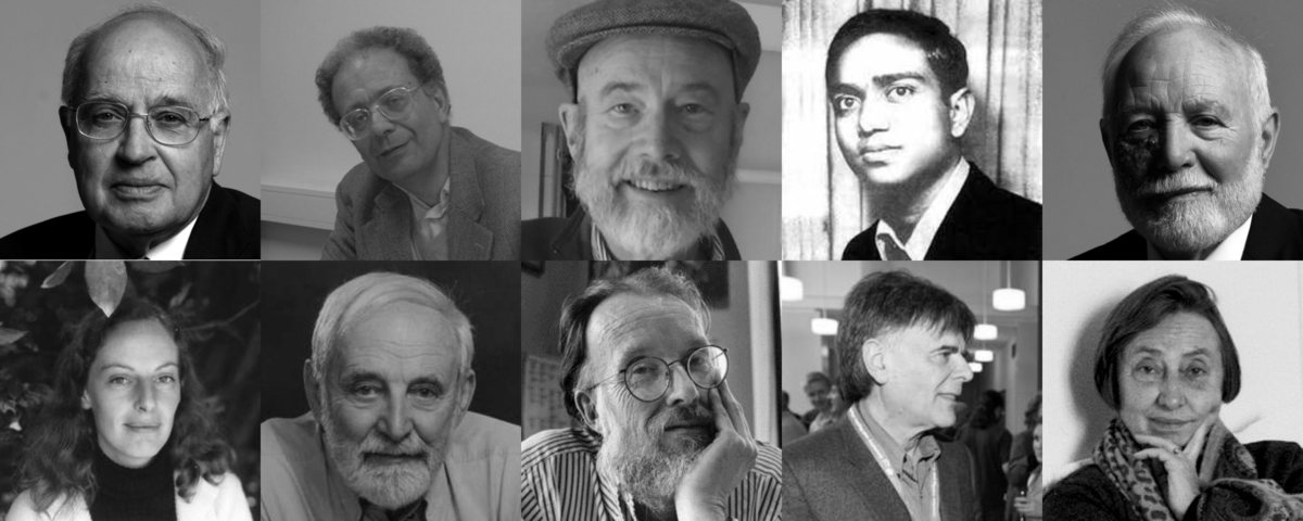
Apropos Gods: here are some of the folks who have done substantial work on these theorems. (I’m sure having overlooked an other dozen or so.) To match the names with the pictures it can help to know that the concatenation has been done automatically with ImageMagick which leads to an alphabetic order): there is Michael Atiyah, Isadore Singer and Raoul Bott. There is also Henry McKean, Jean-Michel Bismut (heat flow proofs in 1986) and Vijay Kumar Patodi (who collaborated a lot with Atiyah-Singer and Bott) especially in the connection with heat flows. Michele Vergne and Nicole Berline studied index theory in the context of representation theory. The two have written with Ezra Getzler (also displayed) a book on heat kernels and Dirac operators in 1992. More in topology and the geometry of elliptic complexes is is Graeme Segal and Peter Gilkey. Gilkey wrote a textbook about the Atiyah-Singer theorem. When looking at textbooks and literature list, the omission of other people becomes evident. There are lecture notes in textbook form of Richard Melrose from 1992 or lecture notes of Antony Wasserman from 2010. The mother of all expositions is the red booklet SASIT (Seminar on the Atiyah-Singer index theorem, by Richard Palais) from 1965 which starts with a nice intro article by Armand Borel and then has various chapters by Robert Solovay, Richard Palais, Robert Seeley, Edwin Floyd and Weishu Shih. There is also the 1978 textbook of Patrick Shanahan. On the historical side, there is the article of Loring Tu who calls a precursor of Atiyah-Bott the “Woods Hole fixed point theorem” named after the Cape Cod place, where a conference took place in 1964. Tu also mentions the influence of Goro Shimura in that matter. By the way, this short historical article of Tu contains a nice expositions for a more general audience on Lefschetz fixed point. Tu was collaborating both with Shimura and Bott. Tu also mentions the influence of other mathematicians at that conference like Jean-Louis Verdier, David Mumford or Robin Hartshorne.

Already Gauss-Bonnet, telling that integrating a suitably normalized curvature over a surface always leads to the Euler characteristic, or the Brouwer fixed point theorem telling that a continuous map from a disc to itself has a fixed point are marvelous. Gauss-Bonnet generalizes to arbitrary dimensions in the form of Gauss-Bonnet-Chern while Brouwer generalizes to a Lefschetz fixed point formula. How is it possible to top these milestones, these mountain peaks? One could think of enlarging the geometric objects or maps, but quantum mechanics points to operators and suggest to generalize the operators which are involved. In the case of Gauss-Bonnet or Brouwer-Lefschetz one deals with the de-Rham complex an elliptic complex involving vector bundles. It is in physics that more general vector bundles are studied, especially in the context of particle physics, where gauge fields describe forces.

The starting point is that one can write the Euler characteristic as the analytic index of an elliptic operator . The space E is the vector bundle of even forms and F is the vector bundle of odd forms. The operator is the Dirac operator defined by the exterior derivative d. The dimension of the kernel of D is the intersection of the kernels of and which is the dimension of the Harmonic forms which by Hodge is the sum of the dimension of the even cohomology groups. Similarly, the dimension of the kernel of D^* is the sum of the dimensions of the odd cohomology groups. The analytic index is therefore the Euler characteristic.

On the dynamical level, the Lefschetz number is a super trace of an linear operator acting on the cohomology. This can be generalized by replacing the de Rham complex by an arbitrary elliptic complex and again look at the super trace of the induced map on cohomology. This should then again be a sum of indices, summing over the set of fixed points. Also this is in the continuum a bit technical as one has to make sure for example that there are only finitely many fixed points as otherwise one has to say how to integrate over the fixed point set. It turns out that for the identity map, where every point is a fixed point, every point contributes and it is the curvature which captures this. In some sense, Gauss-Bonnet is a special case of Brouwer-Lefschetz, but in the continuum, that is less evident.

It turns out that both Gauss-Bonnet and Brouwer-Lefschetz are quite easy to formulate in the discrete. In particular, we can enjoy the absence of any technicalities: on finite abstract simplicial complexes, all the operators are finite matrices and every little detail can be implemented faithfully on a computer as all curvatures are rational numbers, all indices are integers etc. Having no technical difficulties makes it easier to focus on the underlying ideas.

Gauss Bonnet, prototype for Atiyah-Singer This theorem tells that if take a graph equipped with the Whitney complex so that the Euler characteristic is where x runs over all complete subgraphs and , then summing up the curvature over all vertices of the graph gives . The integers are the k-vertex degrees of the vertex x. It counts the number of (k+1)-dimensional simplices x in G which contain v. The proof of Gauss-Bonnet is almost tautological: think of as a curvature on simplices and the definition of Euler characteristic as a Gauss-Bonnet formula already. Now distribute equally to each of the dim(x)+1 vertices v in x. The curvature K(v) is what has reached the vertex v. The result generalizes to an arbitrary simplicial complex G: let V be the set of vertices (zero dimensional sets in G), then the curvature which defines the Euler characteristic can be distributed from each simplex equally to its vertices. The same curvature formula now applies, where are the number of dimensional simplices containing v.

Brouwer-Lefschetz, prototype for Atiyah-Bott If we take a graph endomorphism T which has the cohomology of a ball, then there is a simplex x fixed by T. It is a consequence of a fixed point formula: define the index of a fixed simplex as , where is the signature of the permutation which T induces on x. The fixed point formula tells in that case that as 1 is the Lefschetz number. Again, one can push the index from simplices to vertices and call a vertex $v$ a fixed point if it is mapped into a simplex containing v. If T is the identity, the index on simplices is and the index on vertices is the Euler curvature K(v). The proof is a heat deformation argument. The exterior derivative d defines and the Laplacian . The key observation is that the super trace of is t-independent. For , we get the super trace of restricted to fixed points and for we get the super trace of acting on harmonic forms rsp. cohomology.

We see that in both cases, there are just two ingredients: the quantity under consideration is linked to cohomology on one side and then linked to curvature or index data linked to the zero dimensional parts (points) of the space. We did not mention Euler-Poincaré in the Gauss-Bonnet case but integral geometry allows to see Euler-Poincaré as as special case of Gauss-Bonnet.

Having trivialized Gauss-Bonnet and Brouwer in the case of the traditional de-Rham complex, one can look at more complicated complexes. What do we really need to prove these theorems? In order to link the combinatorial data with the cohomological data one only needs a McKean-Singer symmetry telling that the nonzero eigenvalues of D² on the even are the same than the nonzero eigenvalues on the odd forms. The connection of the combinatorial data pushed to the vertices works very generally for valuations or multi-linear valuations. But most valuations are not topological in nature. It is the McKean-Singer symmetry which allows to translate the quantity into something cohomological and so more robust.

The discrete Atiyah-Singer or Atiyah-Bott generalizations rewrite these theorems for discrete elliptic complexes. One can worry that there are no interesting examples beyond the de Rham complex but there are. We will look after that at connection complexes, whicih are more general and where the Wu characteristic generalizes the Euler characteristic. Then there are product complexes which are not simplicial complexes as described in the ring paper.

Example 1: de Rham complex

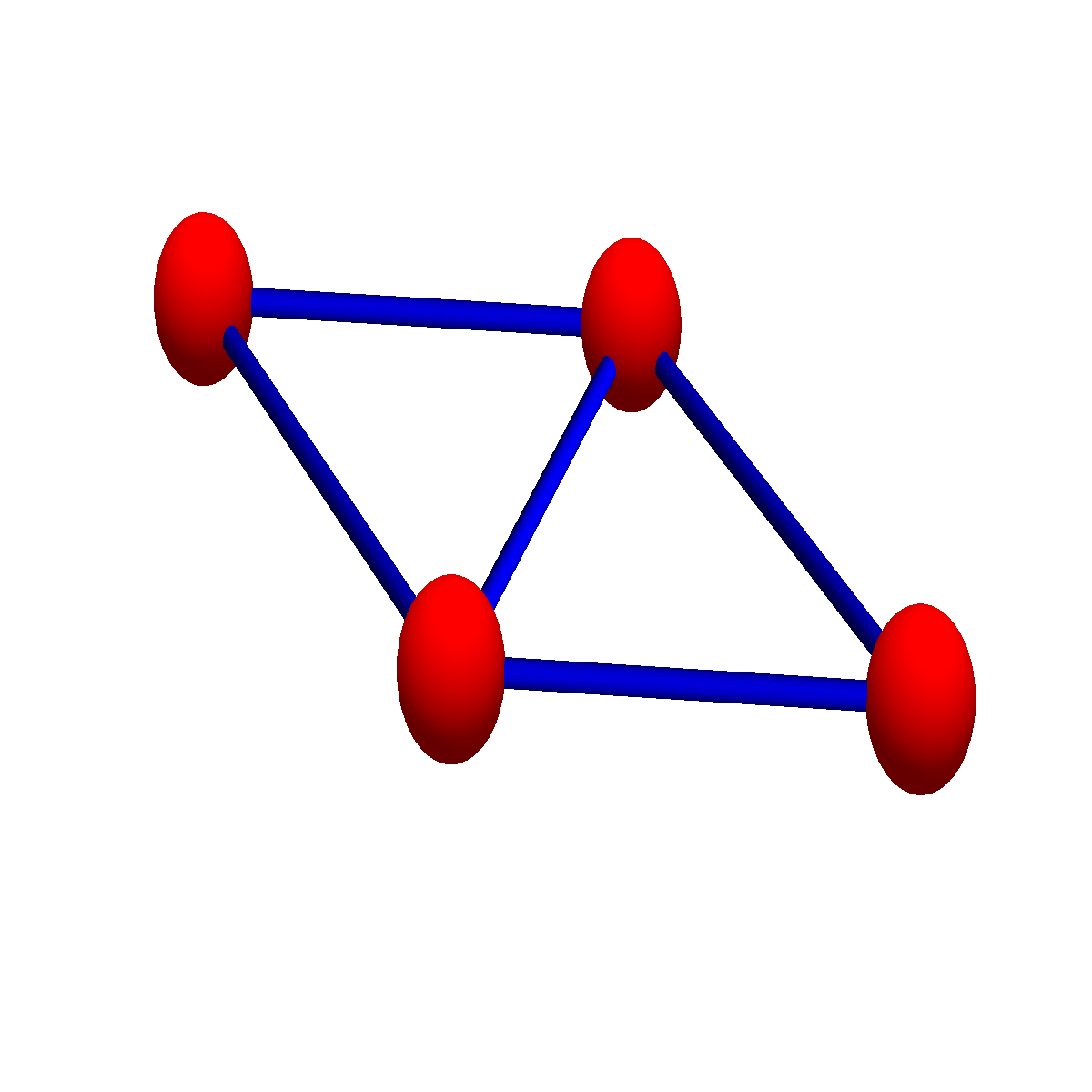
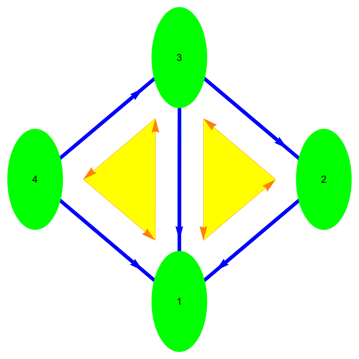
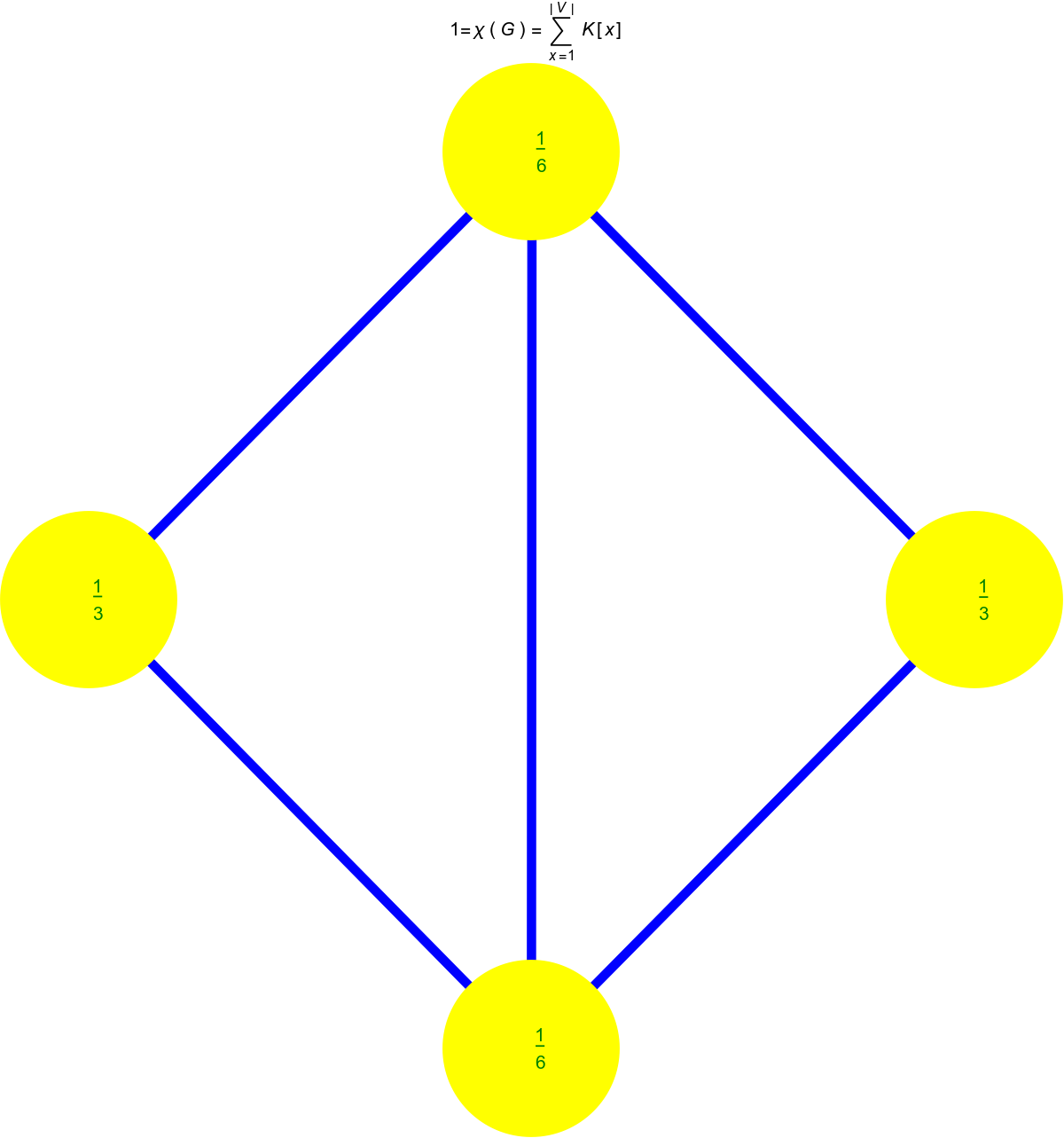
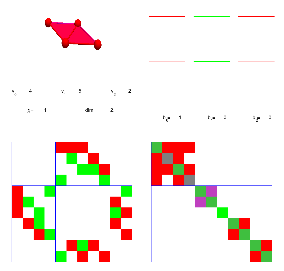
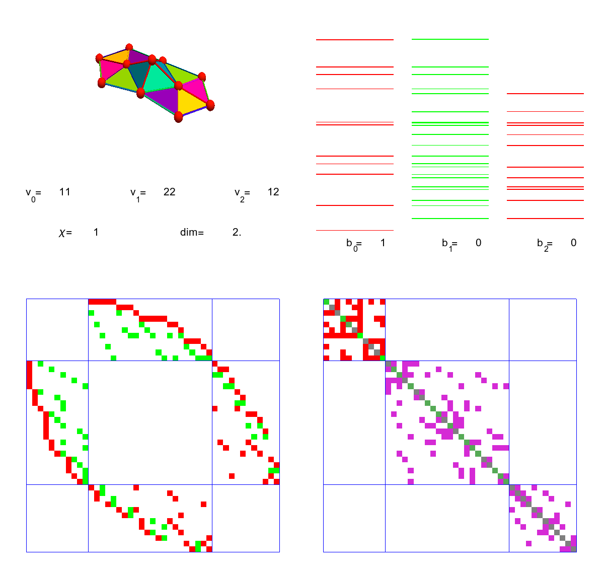
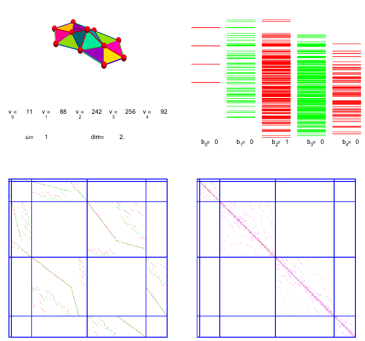
Lets take a concrete simplicial complex. It is the Kite graph G={{1, 2, 3}, {1, 3, 4}, {1}, {2}, {3}, {4}, {1, 4}, {1, 2}, {1, 3}, {2, 3}, {3, 4}}. The first picture shows the graph, the second indicates the simplices in it, the third attaches the curvature K(v) to the 4 vertices. In this two dimensional case, this is just K(v)= 1-V0/2-V1/3, where V0 is the number of vertices in the unit sphere and V1 is the number of edges in the unit sphere. The last picture shows the Dirac operator D and the Hodge Laplacian D² as well as the eigenvalues of the blocks. Since the graph is contractible, there is only one harmonic form, the constant 0-form leading to one single eigenvalue 0. The other eigenvalues are paired showing the Mc-Kean Singer super symmetry. The first block of the Hodge Laplacian, which is the usual scalar Laplacian in calculus has eigenvalues {4,4,2,0}. The second block on 1-forms acts on F has the eigenvalues {4,4,4,2,2}, the last block on 2-forms has the eigenvalues {4,2}. The first and third block act on E, the space of even forms. The index of the Dirac operator D:E=R^6 -> F=R^5, is dim ker D – dim ker D^* = 1-0=1. Notice that we have drawn the Dirac operator as a 11×11 matrix acting on ExF. If it is seen as a map from E to F, it is a 5×6 matrix. You can see this matrix by looking at the first and third block in the second row of the 11×11 matrix. As in finite dimensions, the index of a nxm matrix is always m-n, we can write the index also as 6-5=1, which is the definition of Euler characteristic, as there are 6 even dimensional simplices and 5 odd dimensional simplices. It is this almost tautological “boredom” of the index in finite dimensions, which initially prevents to associate it with index theorems (which are deeper and buried behind a pile of functional analysis). An other stumbling block why the association to finite dimensional situations does not immediately come to mind is that in the continuum, given a family of elliptic operators D(t), then because the index is finite and is continuous, it has to be constant. We can not argue like that in the discrete as deformations like homotopy deformations are done in jumps. In the case of the de Rham complex as just described, everything is homotopy invariant. But we will look in a moment at the connection complex, an other elliptic complex, where the homotopy stability does no more hold and which leads to finer invariants allowing to distinguish homotopically equivalent spaces like the cylinder and the Moebius strip, which are both homotopic to a circle but are topologically different. One can see them also as two non-equivalent different fibre bundles over the circle.

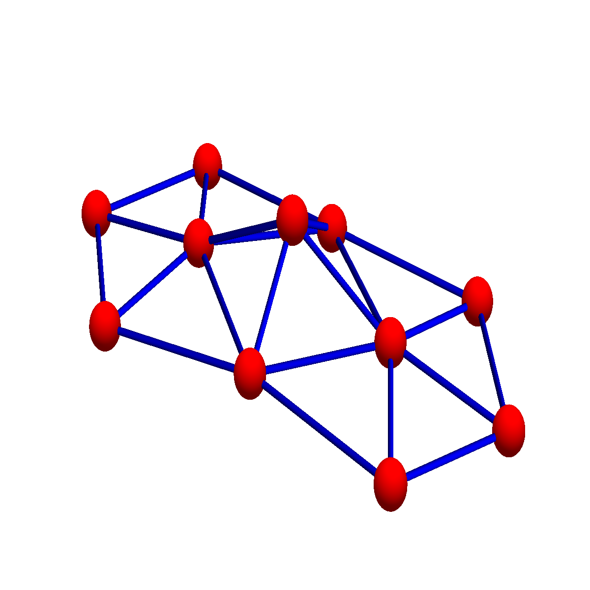
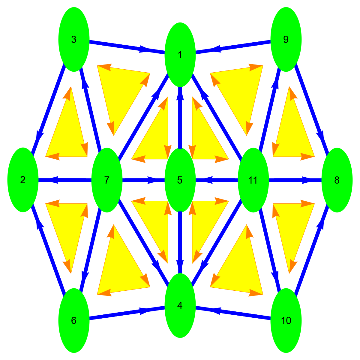
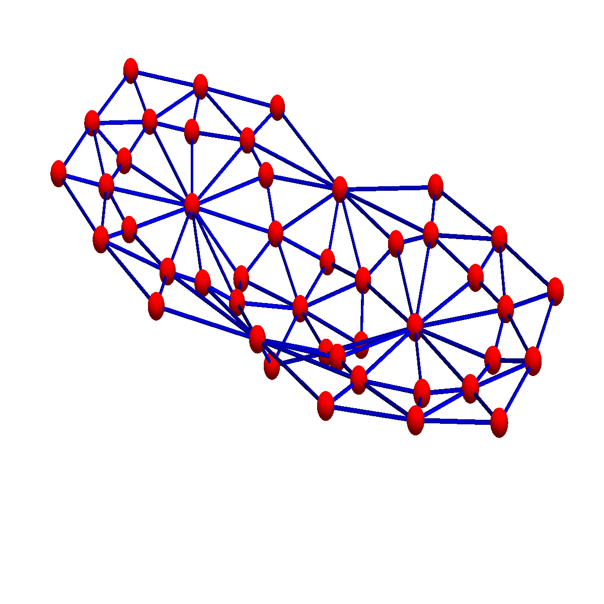
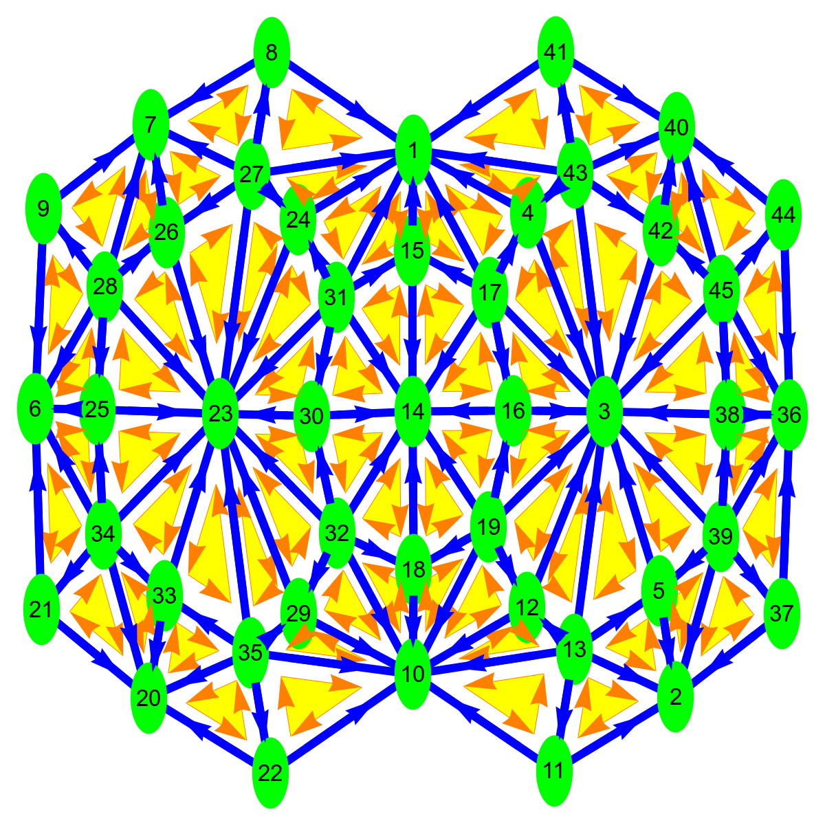
Lets look first at the Barycentric refinement of G. It is the simplicial complex G={{1}, {2}, {3}, {4}, {5}, {6}, {7}, {8}, {9}, {10}, {11}, {1, 3, 7}, {1, 5, 7}, {1, 5, 11}, {1, 9, 11}, {2, 3, 7}, {2, 6, 7}, {4, 5, 7}, {4, 5, 11}, {4, 6, 7}, {4, 10, 11}, {8, 9, 11}, {8, 10, 11}, {1, 3}, {1, 5}, {1, 7}, {1, 9}, {1, 11}, {2, 3}, {2, 6}, {2, 7}, {3, 7}, {4, 5}, {4, 6}, {4, 7}, {4, 10}, {4, 11}, {5, 7}, {5, 11}, {6, 7}, {8, 9}, {8, 10}, {8, 11}, {9, 11}, {10, 11}}. Again we show first the graph, then indicate the simplices with some orientation (clearly not a compatible orientation even so this would be possible here but it does not matter).

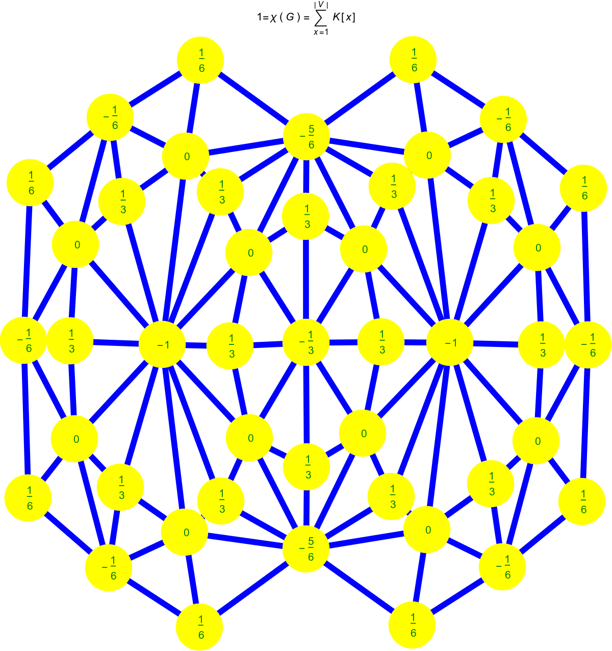
Just for fun, here are the pictures for the next Barycentric refinement G2. You see that the curvatures become more extreme and this indicates that when going to the continuum, not only Barycentric refinements but also some smoothing of the curvature data is needed. In this case, the limiting geometry is a two-dimensional disc with boundary, where the curvature is supported on the boundary. The Gauss-Bonnet theorem then becomes a Hopf Umlaufsatz (which by the way had been my entry point to this part of graph theory). The classical results are always also a bit more technical when manifolds are replaced with manifolds with boundary. In the discrete we don’t care, the complexity is the same whether we have a discrete manifold or a random Erdös Rényi graph.

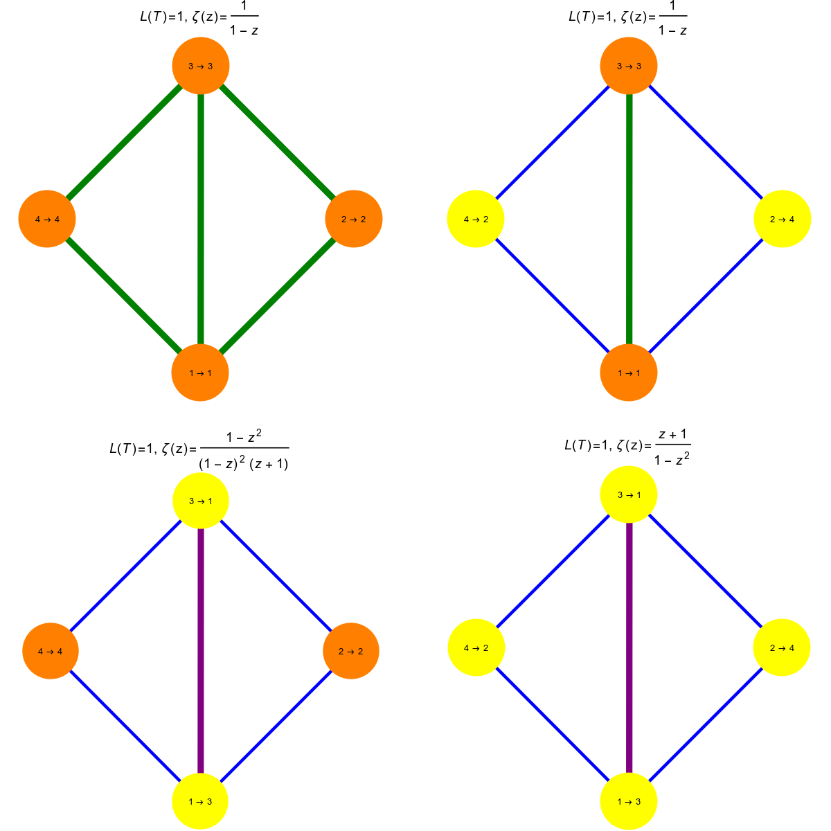
Now to Atiyah-Bott still in the de Rham case, where it is the Brouwer-Lefschetz fixed point theorem. Here is a picture from the Lefschetz article. It shows the situation for the 4 automorphisms of the graph. In each case, the fixed simplices are colored differently. For each transformation, there is also the Zeta function (a Ruelle zeta function close to the Artin-Mazur zeta function). In any case, the simplicial complex has a trivial cohomology which means that the Lefschetz number is 1. There must be a fixed simplex therefore. In the identity case, every of the 11 sets in the simplicial complex G is a fixed point, in two of the reflection cases, we have three fixed points, an edge and two vertices. There is one automorphism (the last one) which has only one fixed point. It is the edge joining the two triangles. In that case the Brouwer index of that edge is 1 as it has odd dimension and the permutation T induces on it has signature -1.

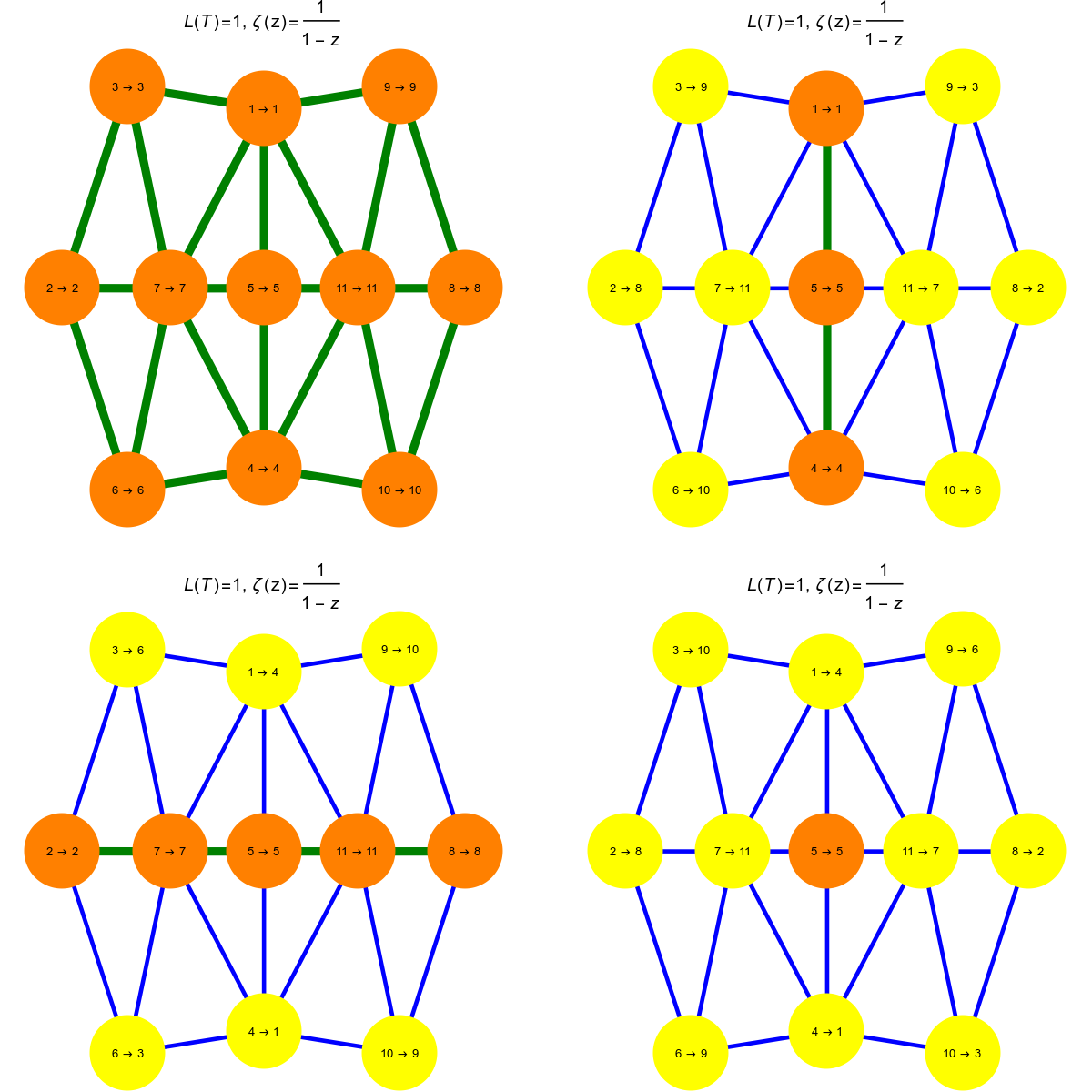
Here is a similar picture for the Barycentric refinement. The Automorphism group is the same, it is generated by two reflections, if when composed produces a reflection at the origin (shown in the fourth picture). The fixed point in that case is now not an edge but a vertex. A fixed vertex always has Brouwer index 1. A fixed edge can have Brouwer index 1 or -1, depending whether the edge is flipped or not.

Example 2: Connection complex

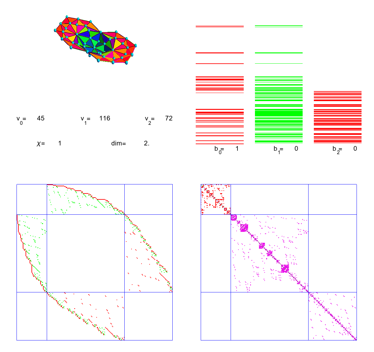
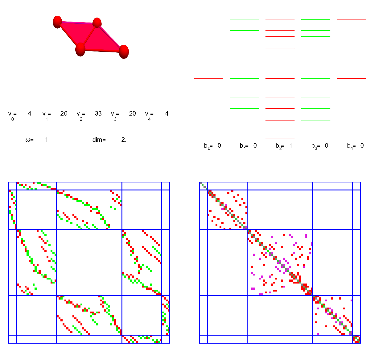
Lets look at a less familiar elliptic complex. The underlying geometric object is still the kite graph G. But now E_k is the set of (a+b=k)-forms, functions on pairs of intersecting simplices of dimension a and b. The next picture illustrates the story in one swoop. For k=0, there are just 4 pairs, the interactions of the 4 zero dimensional parts of space. For k=1, there are 20 pairs of interactions between a zero dimensional part and a one dimensional part. Then, for k=2, there are 33 pairs. It consists of interactions of 1-simplices with 1-simplices or interactions between 2-simpices with 0-simplices. Then there is a 20 dimensional interaction space adding up dimensions to 3 and finally a 4 dimensional space of interactions of the two triangles, two self-interactions and two interactions between the different triangles. the picture shows the corresponding Dirac operator D and its square, the interaction Laplacian. We see also the cohomology. The only Betti number which is non-zero is b_2. The alternating sum of these Betti numbers is the Wu characteristic.

One part of the discrete Atiyah-Singer theorem now tells just that 4-20+33-20+4 = 0-0+1-0+0. This is the identity about the analytic index. The second part will relate that with a sum of curvatures. We will look at this afterwards.

Here is the situation for the Barycentric refinement. The Betti numbers have not changed but the number of interaction pairs have. We still have 11-88+242-256+92=1. You still can clearly make up the supersymmetry present in the spectrum. There are lots of eigenvalues but the differential complex is an elliptic complex.

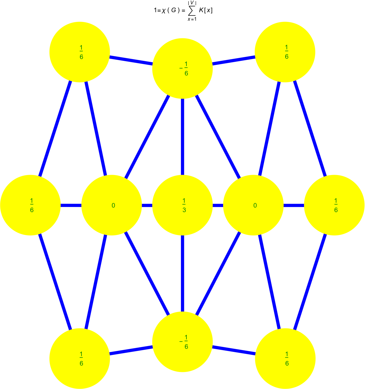
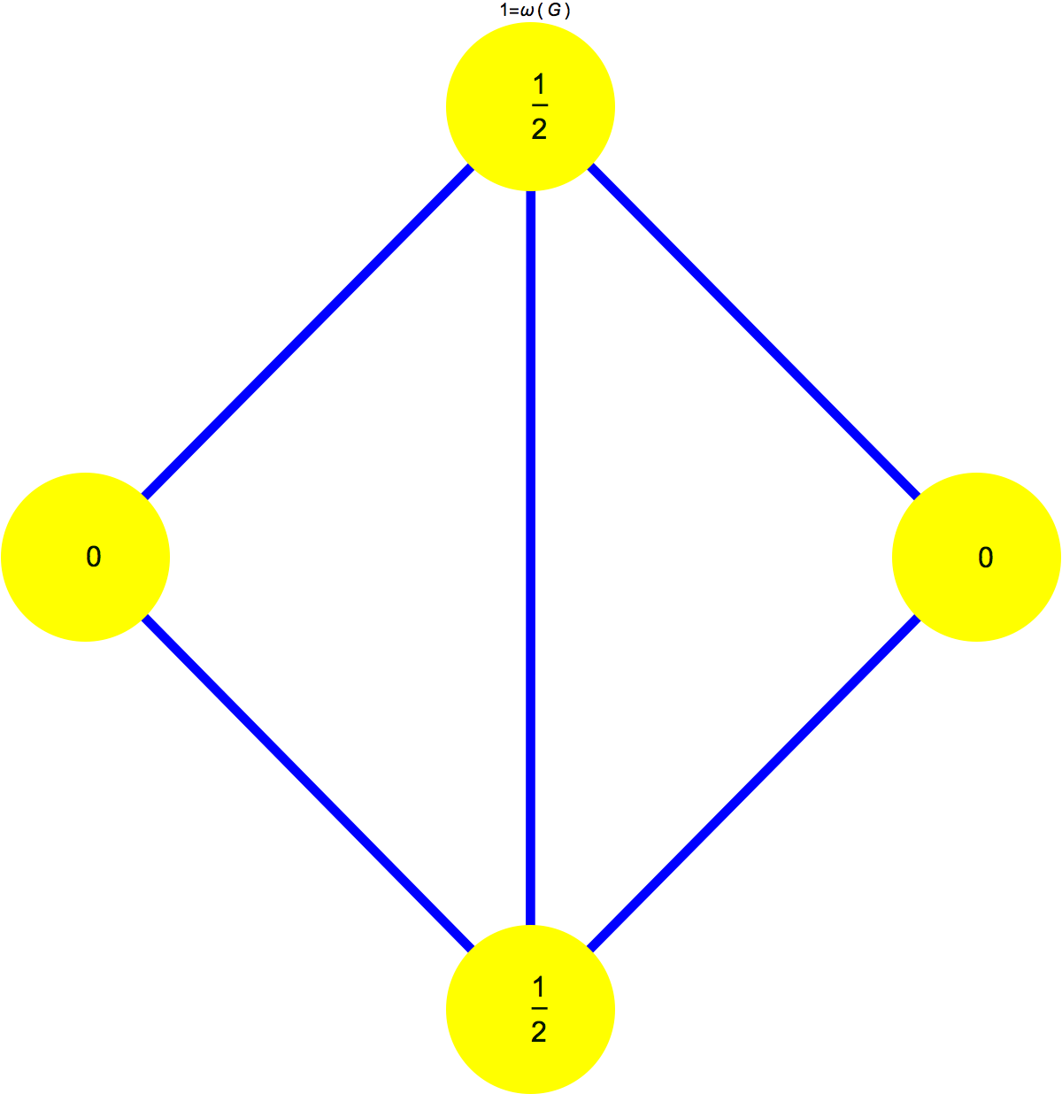
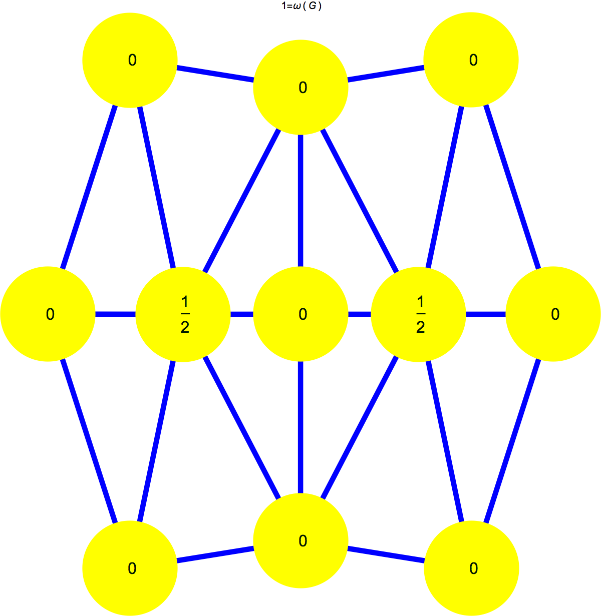
Now here are the Wu curvatures. As in the case of Euler curvature, they are obtained by pushing the simplex curvatures equally down to the vertices. To the left we see the Kite graph, to the right its Barycentric refinement.

Example 3: Deformation of de Rham complex

A natural way to generalize the de Rham complex is simply by deforming it. The idea of deforming the differential complex is not new. A famous example is the Witten deformation which was used to prove the Morse inequalities. The Witten deformed Laplacian is with , where f is a Morse function. It has the effect to move the interesting stuff of the eigenvectors towards the critical points, where one has harmonic oscillators. To cite Cycon-Froese-Kirsch and Simon (a book from where I learned this as a student): this is the quasiclassical eigenvalue limit. The asymptotic estimates for the eigenvalues of L(t) can be used to estimate the dimension of the kernel of L(t) on p forms. The number of eigenvalues obeying is , the number of critical points with Morse index p, one has .
While the Witten deformation is a deformation of the differential complex, we look at a more exciting deformation. Actually, it does not lead to a deformation of the Laplacian as L(t) will stay the same. But it will produce a deformation of the exterior derivative and Dirac operator. The Dirac operator will have the form , where is a diagonal term which grows. The Connes distance defined by increases so that this deformation describes an expansion of space. part of space is fed into a diagonal “dark matter” part b(t) which takes over more and more. This all happens under the hood. We don’t see it classically when looking at the Laplacian only as the Laplacian L(t)=D(t) D(t)^* stays untouched. (One can easily show that L(t) stays constant because L’=[B,L] and BL-LB can be shown to be constant zero.). Also exciting is that this dynamical system is an integrable Lax deformation , where . It is a basic property of this system that it expands with an inflationary start, like in cosmology. Unlike in cosmology, where people put in expansion through a “deus ex machina” device, the inflation which happens here is a mathematical consequence by just letting the geometry move freely in its isospectral set. It is inevitable. Lets look at his in detail with the simplicial complex of the kite graph.

We first look at the deformation D=d+d^* + b, B=d-d^*. The left hand side shows the Dirac operator D(t), the right hand side the unitary U(t). One can see that d(t) goes to zero very fast. The b part is asymptotically an operator which is the square root of L but has the same block structure than L. The unitary conjugation U(t) converges to the fixed matrix. We are in a scattering situation like the finite non-periodic Toda lattice.

M4V,
Ogg,
Webm.

Now we look at the deformation D=d+d^* + b, B=d-d^* +i b. The left hand side shows the real part of the Dirac operator D(t) and the right hand side the real part of the unitary U(t) which conjugates D(t) to D(0). What happens now is that the off diagonal part of the Dirac operator continuous to oscillate but still shrinks exponentially. If B is the asymptotic which is also a square root of L, then the asymptotic Schrödinger evolution is given by the unitary exp(i b t). Now, what is nice in the discrete that the Schrödinger evolution of the Dirac operator is nothing else than the wave evolution for the Laplacian. If we write and the wave as (with pseudo inverse of D), then the wave is the solution of the wave equation for the Laplacian . There appears to be a paradox as does not move under the deformation. How is the wave equation then affected by the deformation of the differential complex? It is through the link of position and velocity. The velocity part of the wave gets changed which is an other way to express that the distance in the geometry changes. It was Alain Connes who seems have realized first that all Riemannian geometry is encoded in the elliptic complex. The Riemannian metric is actually already defined by d_0, the gradient through the Connes distance . Why use such a seemingly complicated way to measure distances? For Connes it is a way to generalize the geometry to non-commutative situations like in topology where the C^* algebra of continuous functions is replaced by an arbitrary C^* algebra or in measure theory, where the von Neumann algebra of bounded measurable functions is replaced with a general von Neumann algebra. We see here that it is also useful in the discrete to delegate the distance measuring to the elliptic complex. If we deal with a finite object like the kite graph, then how do we measure distances? One way is to look at the geodesic distance between two points. This is rigid. How would you place more general “Riemannian geometries” on such a space. One could artificially define different distances between the nodes but that is not natural. Much better is to look on how distances are measured in the first place in nature. It is now not only on the macro scale (with telescopes) or microscopes (e.g using electron microscope) but also on the meso scale (i.e. using laser distance measuring devices) that we use light to measure distance. Since the speed of light is fixed, light (solutions of the wave equations) is a great yard stick. This can also be done in the discrete and Connes distance essentially does that. So, when deforming the exterior derivative (like gradient) like in the Witten or Lax deformations, then we deform the distances. Here, because d(t) goes to zero, space expands.

[The story of the experimental discovery of expansion of space is interesting: It was Edwin Hubble and Goerge Lemaitre have independently found evidence for that and did the data fitting estimating the expansion rate. (Lemaitre in 1927 and Hubble in 1929). Le Maitre was both a mathematician (PhD under guidance of de la Vallée Poussin) and cosmologist (PhD under guidance of Arthur Eddington and Harlow Chapley. The story is well told in the book of Lydia Bieri and Harry Nussbaumer with an extended abstract here on the ArXiv. Some more light into the story brought a letter of Le Maitre discovered recently: see this Nature article of Mario Livio from 2011.]

But lets go back to the system (which is just a mathematical model featuring an exponentially expanding geometry). Here is the numerical computation of the evolution of D(t) (left) and real part of U(t) to the right. It is not very spectacular. But one can see how the kinetic side block parts of the Dirac operator get moved to the center. In the limit, the operator has the same block structure like the Laplacian L=D(t)². While d(t) disappears in the limit, at every finite time t, we have an elliptic complex complex given by exterior derivative d(t).

M4V,
Ogg,
Webm.

One knows since about 20 years that the universe is not only expanding but that its expansion is accelerating (there has recently however appeared more evidence which might question the accelerated picture). An acceleration is compatible with the nonlinear expansion of the Lax system. But it does not show “a cosmic inflation”. The Lax system actually starts slow and the settles to an exponential growth. This happens for any simplicial complex (or Riemannian manifold) except the case when the simplicial complex is zero dimensional in which case there is no expansion. You see a typical situation in Figure 2 of my integrable evolution equation article.

In the note on discrete Atiyah-Singer and Atiyah-Bott result for simplicial complexes, I had mentioned the possibilithy that the deformation could produce “spurious fields” due to the fact that the classical boundary is no more a boundary. But as indicated in the integrable evolution article on the first page, it is not only the intersection of the kernels of and (which are the Harmonic forms) which stay the same but also the cocycle spaces themselves (the kernel of d as well as the kernel of ). So, all these fields are all zero. I foolishly only re-realized this after computing the “forces” numerically and saw them to be zero. Also the deformed boundaries do “enclose” no field sources. Which is much more natural.

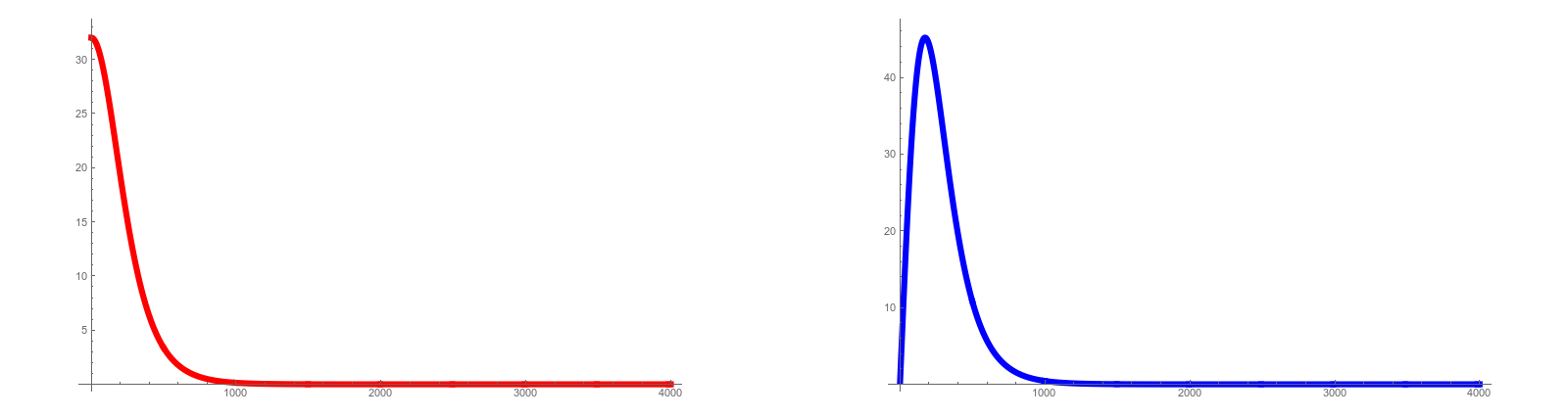
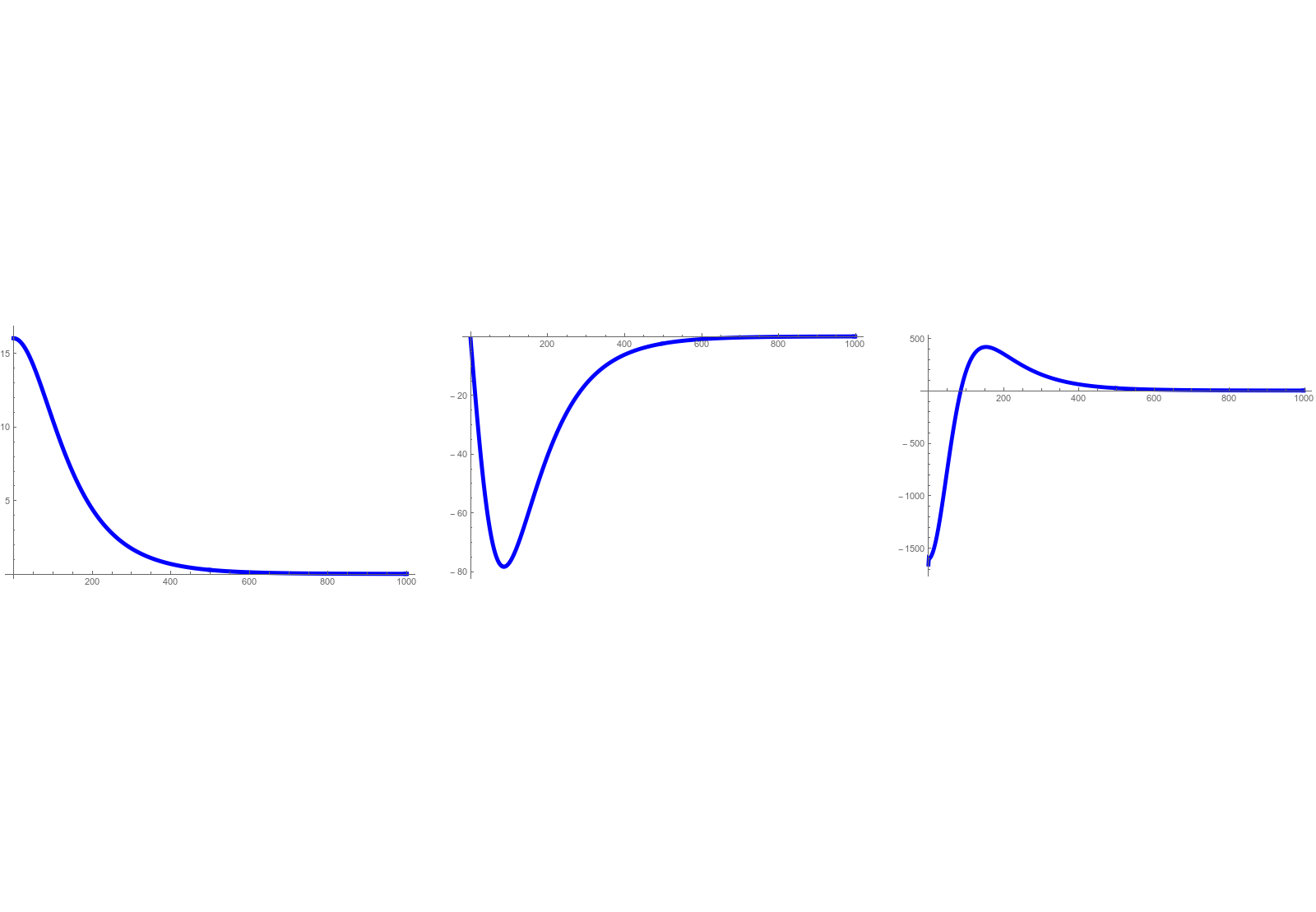
Lets again look at the expansion rate, the same graph as shown in the picture but now for the Kite graph: the first red graph shows tr(M(t)), a measure of the size of , the second blue graph (with a bump) shows d/dt tr(M(t)), where is the Laplacian defined by d(t). The Dirac operator of the deformed exterior derivative is not isospectral to D as it decreases. It is which is. The second picture to the right shows the situation if one choses for , the non-scattering situation, where the asymptotic evolution is a linear wave equation. We see the real part, where a little “echo” bump after the inflation bump. If we look at the the absolute value, then we see a picture almost indistinguishable from the scattering situation where . So, which one is the right one? One should probably see it as a symmetry issue. There is no reason, why an elliptic complex should not become “complex valued”.

We have now “elliptic complexes” over “simplicial complexes” which become “complex valued” but without “technical complexity”.

It is kind of interesting that we start with a finite discrete geometry and let its elliptic differential complex evolve freely in its symmetry group, then a complex structure appear – out of no-where! It is not that we have placed the complex numbers in artificially, we just “allowed” the complex to become complex-valued and it did (true of its nature …). By the way, the “dark matter” or “dark energy” part b(t) stays real (with “real” meaning Re(b)=b). In reality, nobody knows what “dark energy” is. In this mathematical frame work it is a good word, as we don’t really know also what it geometrically means here.

[ Update August 27: having seen that an elliptic complex naturally can involve complex valued entries, one can wonder whether larger division algebras can appear. Is it possible that the operators become quaternion- or even octonion-valued? I think the answer is yes, as this was mentioned in the particles and primes paper. It can be mentioned here too: instead of placing one single elliptic complex onto the geometry, we can place several ones. Mathematically we could look at a sum of elliptic complexes in the sense like fibre bundles are added in K theory. Why not place three complexes in and call the corresponding complex unit i,j or k. What happens is that we have now three complex planes glued together at the real line. Now think about each plane as a “particle generation” (this fits as we know only 3 generations but it is not known whether there are more.) The quaternion picture suggests that there can not be more but that could be as silly as Kepler trying to match the planetary orbits with the platonic solids. Anyway, it is appealing because for neutrini (in the particle and prime allegory, the real primes among the Gaussian primes are the neutrini while the other ones are Lepton pairs) one observes “neutrino oscillations” while for the electrons this is not observed. Now one can wonder why the different flavors have different properties. Well, the Lax deformation we have looked at is one of many deformations. Like higher order Toda Lattices, one can look at higher order Lax deformations. Each is a geodesic in the symmetry group. If we pick three symmetries randomly, it is very unlikely that all are the same, there will be a fastest one (electron, electron neutrino, up and down particles), the second one leads to the second generation (muon, muon-neutrino, charm and strange), the last one finally is the third generation (tau, tau-neutrino, top bottom). Why does the picture not break out to octonions? Because there are only two associative complete division algebras, the complex numbers and the quaternions. Mathematically also relevant is that the unit spheres in these spaces are the only spheres in Euclidean space which are also Lie groups. So, there are purely mathematical pointers (Hurewitz or Frobenius theorems, structure of Lie groups), which indicate why complex and quaternion fields are natural. Number theoretically, there are then some affinities between primes in the complex plane (leptons) and primes in quaternions (hadrons). Looking at equivalence relations in quaternions leads to Baryons and Mesons. This is amusing and most probably irrelevant for physics but it shows that the mathematical structure of the standard model is not that ugly after all as we see similar constructs in combinatorics. ]

The following figure shows the sum for the Dirac matrix . The second and third graph show the absolute value of the first derivative an the second derivative.

[Update: similarly as Toda systems can be used to solve linear algebra problems (for example to diagonalize a matrix and find its eigenfucntions), also the integrable evolution equation for D solves a linear algebra problem:
the operator D(t) converges to a real operator B which is a square root of L=D². While there are many square roots of L, the operator B has the same block structure than L and the spectrum is symmetric . The limiting operator B(t) for t to infinity is minus the limiting operator B(t) for t to minus infinity. The evolution produces an explicit conjugation of D(0) with and , which are all similar matrices. ]

While the expansion happens for all simplicial complexes, we have not yet looked at how the expansion rate depends on the size of the complex. It would be good to know especially what happens for very large complexes.

Update August 26: if you want to try out the deformation yourself, here is completely self contained Mathematica code (no libraries needed). Code has been made available at other places: early on this page and later within the articles like in Dirac operator of graph, or on this blog. What the following lines do is to take a graph and then deform its exterior derivative (given in the form of the Dirac operator). The graphics shows then the rate of change of where is the sum of the absolute values of the entries of a matrix. The value of this number gives the exponential expansion rate of the geometry. The integration of the system is done from t=0 to t=4 with 1000 Runge-Kutta steps. The resulting picture is seen then below. The Mathematica lines might look a bit cryptic. The first part is a translation from graphs to simplicial complexes. We could start with a set of sets instead. The Dirac procedure just builds the matrix D. Then come some self-evident “helper routines” like Runge Kutta. The last dozen lines really contain the computation. In this case, the “3-sphere” is a given as an undirected graph. It is the suspension of the octahedron or (using the Zykov ring language , where $P_2$ is the two point graph without edge). Then the elliptic complex in the form of {DD,br} is computed. The br gives the break points encoding the block structure of D. So, {DD,br} really encodes the elliptic complex. Then we just numerically compute an orbit of D’=[B,D] starting with the Dirac operator . In this case, we have chosen the complex evolution where matrix B(t) encoding the symplecic form is allowed to become complex . The matrix becomes complex too and d(t) d(t) =0 assures that we still have an elliptic complex after deformation. It is essential for the unitary U’ = B U, U(0)=1 that b remains real and this is also the case.

[ There is an other allegory coming in here: while McKean-Singer spectral symmetry is still present, a vector u and its “super partner” D u become exponentially close to each other in the sense that the angle between these two vectors is eponentially small in t. If we would look with a computer at the evolution of a vector u(t), then its super partner v(t) looks the same after a short time. Something like that (of course in a million times more complicated framework) could happen with the missing super symmetry in real physics. It is one of the frustrations of particle physisists and especially string theorists that no super particles are found. Maybe they are just hidden by their brothers … Fortunately, in mathematics and especially in simple frame works like here (combinatorics and linear algebra), we are not concerned with missing super partners. We deal here with geometry of finite sets and dynamical systems in an algebra of finite matrices. The jargon “super symmetry” is used in a mathematical sense as used in the book of Cycon-Froese-Kirsch and Simon for example.]

(* Mathematica code  Oliver Knill May 2013,           *)
(* see https://arxiv.org/abs/1306.0060   for the math *)

ListOfCliques[K_,k_]:=Module[{n,ss,m=Length[EdgeList[K]],s,u,V=VertexList[K],
W=EdgeList[K],U,ll={}},s=Subsets[V,{k,k}]; n=Length[V];
W1=Table[{W[[j,1]],W[[j,2]]},{j,Length[W]}]; If[k==1,ll=V,
If[k==2,ll=W1,Do[ss=Subgraph[K,s[[j]]];
If[Length[EdgeList[ss]]==Binomial[k,2],
ll=Append[ll,VertexList[ss]]],{j,Length[s]}]]];ll];

Dirac[s_]:= Module[{a,b,vl=VertexList[s],l,n,v,m,R,t,d},
n=Length[vl];d=Table[{{0}},{p,n-1}];
l=Table[{},{p,n}];v=Table[0,{p,n}];m=n;
Do[If[m==n,l[[p]]=ListOfCliques[s,p];
v[[p]]=Length[l[[p]]];If[v[[p]]==0,m=p-2]],{p,n}];
t=Sum[v[[p]],{p,n}]; b=Prepend[Table[Sum[v[[p]],{p,1,k}],{k,Min[n,m+1]}],0];
R=Table[0,{t},{t}]; If[m>0,d[[1]]=Table[0,{j,v[[2]]},{i,v[[1]]}];
Do[d[[1,j,l[[2,j,1]]]]=-1,{j,v[[2]]}];
Do[d[[1,j,l[[2,j,2]]]]=1,{j,v[[2]]}]];
Do[If[m>=p,d[[p]]=Table[0,{j,v[[p+1]]},{i,v[[p]]}];
Do[a=l[[p+1,i]];
Do[d[[p,i,Position[l[[p]],Delete[a,j]][[1,1]]]]=(-1)^j,
{j,p+1}],{i,v[[p+1]]}]],{p,2,n-1}];
Do[If[m>=p, Do[R[[b[[p+1]]+j,b[[p]]+i]]=d[[p,j,i]],{i,
v[[p]]},{j,v[[p+1]]}]],{p,1,n-1}];{R+Transpose[R],b}];

UpperTriangular[A_]:=Table[If[i>=j,0,A[[i,j]]],
{i,Length[A]},{j,Length[A[[1]]]}];

UpperDirac[{DD_,br_}]:=Module[{DDD},DDD=UpperTriangular[DD];
Do[Do[Do[ DDD[[br[[k]]+i,br[[k]]+j]]=0,{i,br[[k+1]]-br[[k]]}],
 {j,br[[k+1]]-br[[k]]}],{k,Length[br]-1}];DDD];

RungeKutta[f_,x_,s_]:=Module[{a,b,c,u,v,w,q},u=s*f[x];
a=x+u/2;v=s*f[a];b=x+v/2;w=s*f[b];c=x+w; q=s*f[c];x+(u+2v+2w+q)/6];

s=UndirectedGraph[Graph[{1 -> 2, 1 -> 3, 1 -> 4, 1 -> 5, 2 -> 3, 
2 -> 4, 2 -> 6, 3 -> 5, 3 -> 6, 4 -> 5, 4 -> 6, 5 -> 6}]]; (* 3 sphere *)

{DD,br}=N[Dirac[s]];DD0=DD;
M=1000;dt=N[4/M];NN=Length[DD];

dd=UpperDirac[{DD,br}];BB= dd-Transpose[dd];BBB=BB;LL0=LL;DD0=DD;
ee=Transpose[dd];BB=dd-ee;CC=dd+ee;MM=CC.CC;bb= DD-CC;VV=bb.bb;
NN=Length[DD];uu={};

Do[f[x_]:=BBB.x-x.BBB;DD=RungeKutta[f,DD,dt];
LL=DD.DD;dd=UpperDirac[{DD,br}];
ee=Conjugate[Transpose[dd]];
BB=dd-ee;CC=dd+ee;MM=CC.CC; bb=DD-CC;VV=bb.bb;
BBB=BB+1.0*I*bb; uu=Append[uu,Total[Abs[Flatten[Chop[dd]]]]],{m,M}];

F[x_]:=If[x==0,0,-Log[Abs[x]]];
vv=M*Table[F[uu[[k+1]]]-F[uu[[k]]],{k,Length[uu]-1}];
S=ListPlot[vv]

Th inflation rate starts at 0, then rises rapidly, reaches a maximum and then settles at a constant rate. It is this first flare which one could label “inflation”. I have compared it with “cosmic inflation”, but of course, in our case, this is a caricature: we are in an extremely simple mathematical setting dealing with one of the simplest mathematical objects one can imagine: a finite abstract simplicial complex. There is only one axiom: it is a finite set of non-empty sets which is closed under the operation of taking non-empty subsets. Now, this simple mathematical structure has algebraic structures in the form of the Dirac operator or Laplacian attached and more generally can be equiped with an elleiptic complex. And such a complex has many symmetries. According to Felix Klein, symmetries define a geometry, according to Emmy Noether, symmetries define conservation laws. Now, the conservation laws are the eigenvalues of the Laplacian. The corresponding symmetries are the isospectral deformations of the Dirac operator. Now, (and this is really nice), it is not necessary to postulate “let there be light”. Light appears automatically in the form of the linear wave equation in which the Lax system settles. Asymptotically, the Lax system is a Schroedinger evolution for a complex wave which if written in real form is the solution of the wave equation , where L is the Hodge Laplacian and is the link between initial position and velocity data of the wave with the complex wave. Now, however we deform the system, even if we would run the system backwards, there is always an “expansion of space”. We definitely have an “arrow of time”, even so the evolution is given by a perfectly reversible Hamiltonian system. As indicated in “An integrable evolution equation in geometry”, this works in the same way also for Riemannian manifolds but things are there more technical, as the exterior derivatives becoming pseudo differential operators making an implementation in a computer more difficult (requiring finite dimensional approximations). In the discrete, the numerical computation deals with finite matrices.