Space and Particles - Quantum Calculus

Sets and Simplicial complexes

The definition of an abstract finite simplicial complex as a set of non-empty sets which is invariant under the process of taking non-empty subsets defines one of the simplest structures in the whole of mathematics. There is one axiom only! Usually, textbooks define it slightly differently in that it is a set G of subsets of a finite set V such that any non-empty subset of an element in G is in G and such that every v in V leads to a set {v} in G. Of course the two statements are equivalent as in the first case, we just can define the base set V as the union of all sets in G. The axiom then implies that every singleton set is in G. It is a small detail but there is a difference: the first formulation does not mention the base set V, nor points {x}, sets of dimension zero. It is a point-free formulation. In topology, “pointless topology” is a true generalization of topology. Introduced by John von Neumann, it is relevant for topoi, a generalization of point set theory introduced by Alexander Grothendieck for which there are examples without points. Simplicial complexes which form a structure which appear at first just a tiny bit more interesting than a set of sets without any conditions, but the invariance condition produces a universe of interesting mathematics. Also the insistance of being combinatorial and not realizing the simplex in Euclidean space looks like a minor thing but it is important as the theory of finite abstract simplicial complexes is something a finitist can accept and work with unlike Euclidean space which does not exist for such a purist. But one does not have to be dogmatic but pragmatic; it is simply that staying within a finite frame work can be essential for a computer scientist. There are various flavors of discrete mathematics leading to a bit of a fragmented vocabulary. A graph theorist, a computer scientist, a combinatorics person or an algebraic topologist use different jargon for the same thing. The advantage of a combinatorial setting is that there is less risks of running into some pathology which the continuum is full of.

[Nice sources are the books “counter examples in …” but there popular paradoxa like the Antoine necklace, the Alexandrov sphere, planar Jordan curves of positive area or the Banach-Tarski paradox which prove that “mathematicians either prove the obvious or what is obviously false” (a tongue in the cheek definition of mathematics which a comedian once stated. Actually, (still tongue in the cheek) if you look on youtube in mathematics, this dichotomy is present: popular Youtube movies either deal with the obvious (like Pythagoras, how to differentiate a polynomial or what a graph is) or then the obviously wrong things (like 1+2+3+… = -1/12 or Banach-Tarski telling that one can cut a ball into 5 parts and reassemble them using rotations and translations to get two balls of the same size. Both statements are true, the first infinite sum is $\zeta(-1)$ and the second follows from the axiom of choice) and extremes make up the majority of popular movies. The actual regular mathematics draws less interest … ). ]

Complexes and Graphs

A finite simple graph is a pair (V,E), where V is a set of points called vertices and where E is a set of unordered pairs (a,b) where a,b are different elements in E. A graph is a network in which different nodes can be connected by edges. The word “simple” refers to the fact that nodes can only be connected by one edge and that no self-loops are allowed. If one looks at graph theory books, they mostly treat graphs as one dimensional objects (curves) where the Euler characteristic $\chi(G) = |V|-|E|$ or then, in topological graph theory, where graphs are networks on two dimensional manifolds, where one has also faces and the Euler characteristic is $\chi(G)=|V|-|E|+F|$ . This has historically grown as much of graph theory dealt with planar graphs or graphs on surfaces. Especially the 4-color theorem pushed graph theory enormously. There is however much more to graphs than what meets the eye. It has probably first seen by Whitney who wrote his thesis under the guidance of Birkhoff that graphs have much more structure as they can, in the form of a triangulation of a manifold essentially do anything one wants to do with smooth manifolds. The concept is today known as the Whitney complex of a graph. If (V,E) is given, let G be the set of subsets A of V, such that in A all nodes are connected to each other. In graph theory, such a set is called a face, simplex or clique, always depending whether the author comes more from network theory (cliques of friends in a social network), from topology (simplices) or from combinatorics (faces). The Whitney complex is one of the possible simplicial complexes one can have on a graph. It is like when looking at various topologies or sigma algebras on a set, one can also look at various simplicial complexes on a set. A graph theoriest probably mostly looks at the 1-skeleton complex $V \cup E$ which treats the graph as a one dimensional structure. One sees this when authors in geometric graph theory talk about homeomorphisms: they build the Barycentric refinement of the 1-skeleton only. A common definition in topology is also to see a graph as a “one dimensional simplicial complex”.

Why graphs

So, why look at graphs then rather than simplicial complexes? Because they are easy to understand. We look at street maps, use graphs as diagrams to explain complicated concepts etc. Simplicial complexes are harder to swallow. One has to appreciate first the concept of a set. History has shown that there was heavy resistance at first when Cantor introduced his “paradise”. In the 60ies (Sputnik shock!) one has tried to make it more accessible. Look at this game for example which a student from one of my E-320 classes has shown me once. I think that if you are able to understand the 100 page manual and rules for this game you are really good. Set theory has entered elementary school during the sixties. Back to the relation between graphs and simplicial complexes. Obviously, graphs (with Whitney complex) only form a subclass of simplicial complexes. But there is not much lost as the Barycentric refinement of an arbitrary simplicial complex is always the Whitney complex of a graph. What is the Barycentric refinement. It is the subset of the power set 2^G for which every element A has the property that all its sets are contained in each other. It is obviously the Whitney complex of the graph $(V,E)=(G, \{ (a,b) \; | \; a \subset b \; {\rm or} \; b \subset a\})$ . So, there is a natural graph G₁ associated to any simplicial complex G. An other important graph is the connection graph G’ of G. It has again G as the vertex set but connects two different vertices a and b, if a and b intersect in a non-empty set. The connection Laplacian is the matrix for which L(a,b)=1 if a and b intersect and L(a,b)=0 else. It is an important matrix as L is unimodular.

Valuations and Integral Geometry

So, what can one do with simplicial complexes? First of all there is a lot of combinatorics. The f-vector f(G) of a complex G encoding the cardinalities of the sets generalizes counting. Given a vector X, the map $G \to <X,f(G)>$ is called a valuation and generalizes counting or Bosonic integration. This is what in calculus appears when computing length, area or volume. The theory of valuations on simplicial complexes is the discrete analogue of integral geometry. There is a discrete Hadwiger theorem of Klain and Rota for example which tells that the set of valuations, abstractly defined as functionals on the lattice of simplicial complexes satisfying $X(G \cup H) + X(G \cap H) = X(G) + X(H)$ has the dimension of the clique number of the complex which is one plus the maximal dimension of the complex. Now, it is a bit disappointing that unlike for sets, where we have a ring with symmetric difference as addition and intersection as multiplication, for simplicial complexes, the lattice given by intersection and union does not lead to a Boolean ring. Take the complex G=K₂=xy+x+y for example and H=P₂ = x + y, where we have already described the complex using Stanley-Reisner polynomials. Now the symmetric difference $G \Delta H = xy$ is not a simplicial complex any more. This was mentioned in in this paper where we extended linear valuations to multilinear valuations. The lack of a ring structure also bothered us when attempting first to prove the unimodularity theorem using algebraic constructs. After months, we decided to extend the category of simplicial complexes to discrete CW complexes, a construct well known in algebraic topology and easy to work with inductively as adding cells is simpler than adding a point to a simplicial complex (which in general adds a plethora of cells simultaneously and which is hard to analyze).

Calculus and Geometric Measure Theory

We have written about this before: calculus not only has a Bosonic version where simplices, the sets in a simplicial complex, are oblivious to orientation. There is also a Fermionic version, where the orientation matters. Most of calculus deals with this but calculus textbooks do not distinguish this which is of course ok as it would confuse. But one has to be aware that computing a surface area integral is a different thing than computing a flux integral. For the surface area the orientation does not matter, for the flux integral it does. A discrete differential form is a function on an oriented simplicial complex which is anti-symmetric in the sense that for any set A in G, f(-A)=-f(A). We have just written -A for the simplex A in which the orientation has switched. (Actually this already defines negative simplices as we need for exstending the monoid of simplicial complexes to a group, but more about this later). How do we get from a simplicial complex G to an oriented simplicial complex? It turns out not to matter. Picking initially some orientations for the simplices is like choosing a basis in Euclidean space. Two different orientations lead in algebraic settings just to a change of basis. Interesting notions like Laplacians don’t depend at all on the choice of the orientation. So, lets assume to have picked an arbitrary orientation. One can implement that also on the Stanley-Reisner picture by modding out xy+yx rather than xy-xy. Any simplex A in G has now a boundary dA. If $A=x_1 x_2 \cdots x_d$ in the Stanley-Reisner ring, then $dA=\sum_{k} (-1)^k x_1 x_2 \cdots \hat{x}_k \cdots x_d$ . Is easy to see that the boundary of a boundary is empty. Define the exterior derivative d on differential forms as df(A) = f(dA). One can extend this to arbitrary subcomplexes of the complex and get Stokes theorem, the fundamental theorem of calculus. One gets close to the continuum situation if the complex is a triangulation of a manifold with boundary and the orientation of the simplices is inherited from the orientation of the manifold. In that case, the boundary of the complex is a triangulation of the boundary of the manifold and we get to the classical Stokes theorem. Yes, it is that simple. If you look at calculus books which do differential forms seriously like Edwards or Abraham- Marsden-Ratiu (my favorate which I essentially followed in this course), then you notice that the vast majoriy of the framework in the continuum is just building up the language and then especially working in a smooth setting making sure that the discrete approximations (Riemann sums and difference expressions) converge in the limit. The core ideas are in the discrete, the rest is more or less technical necessity. Calculus in the continuum generalizes by dualization to measure theory. This requires the language of Schwarz distributions and leads to geometric measure theory, the Fermonic sibling of integral geometry, the Bosonic version. Anyway, we have seen that what we teach in multivariable calculus in weeks culminating in the theorem of Green,Stokes and Gauss is almost a tautology for simplicial complexes. It is actually surprising that this discrete calcululs theory (which was found in its essence already 150 years ago) has not been discovered already by the Greeks. Byt they lacked two essential things: the concept of a function as well as the concept of sets (which by the way was not well received initially even in the 20th century and drove Cantor into the mental institution).

Cohomology and Duality

With an exterior derivative d, one immediately gets cohomology. One first defines cocycles as the elements in the kernel of d and coboundaries as the elements in the image of d. As the square d² is zero, the image of d is contained in the kernel of d. One can therefore look at the quotient space ker(d_k)/im(d_k-1) which is called the k-th cohomology group of G. Its dimension b_k(G) is the k’th Betti number. Similarly as one can encode the f-vector into a function as $e(x)= \sum_{k=0}^{\infty} f_k x^k$ (the Euler polynomial) one can encode the Betti numbers as a function $p(x) = \sum_{k=0}^{\infty} b_k x^k$ (the Poincaré polynomial). The Euler characteristic is defined as e(-1). The cohomological Euler characteristic is defined as p(-1). The Euler-Poincaré theorem is (essentially by the rank-nullety theorem as realized first by Benno Eckmann) tells that the Euler characteristic is equal to the cohomological Euler characteristic. (See my Lefschetz paper for the simple proof of Eckmann). All this holds for a general finite abstract simplicial complex G. Cohomolgy is important as it gives combinatorial invariants of the complex, numbers which do not change when doing a Barycentric refinement. In geometric setups, there is Poincaré duality, if the unit spheres are topological spheres, then $b_0,b_1, \dots , b_d$ is a palindrome. We see that the innocent looking structure of an abstract finite simplicial complex leads to the three basic pillars of combinatorial topology (according to Dieudonné): Barycentric refinement, incidence matrices and duality. Now, locally Euclidean spaces appear a bit special when looling at the large class of simplicial complexes, but it is not as strange as manifold structures appear when “dimension” collides with “homotopy”. Dimension alone does not guarantee Euclidean structure as a tree shows. The unit spheres in a tree are graphs without points so that the three is one dimensional and trees are also homotopic to a point. But if this is combined and if we insist that the unit spheres are spheres (complexes which when punctured become contractible), then only circular graphs remain as connected components of one dimensional structures. Homomtopy and dimension have entered the definition of what a “sphere” is. In the discrete, geometry is essentially sphere geometry as we do not have any concept of lines or planes. Spheres however behave nicely and compensate for the missing tangent spaces.

Homotopy and Spheres

There is an important other aspect which enters when looking at simplicial complexes which correspond to manifolds and satisfy Poincaré duality: the concept of homotopy as introduced by J.H.C. Whitehead. Whitehead was not only a great topologist, he also helped breaking the Enigma code at Bletchley park. He created the important notion of CW complex which is now introduced in any algebraic topology course. It can also be adapted to the discrete for simplicial complexes(after one has has defined what a sphere is). Now it is here where it is better to work with the Barycentric refinement of a complex as it allows to use the more intuitive notion of graph theory to be used. The unit sphere of a node in a graph is the subgraph generated by all the vertices attached to the node. It is again a graph. A graph G is called collapsible if there exists a node v for which when this node (and all connections to it) are removed, the remaining graph is collapsible and for which the unit sphere S(x) of the node is collapsible. The inductive notion of collapsible starts with the assumption that the one point graph is collapsible. A homotopy step is the process of removing a vertex with collapsible unit sphere or then a cone extension over a collapsible subgraph. A graph is called contractible or “homotopic to the 1-point graph” if one can find a sequence of homotopy steps which brings the graph to the 1-point graph. Two graphs which can be transformed into each other by homotopy steps are called homotopic. A graph is a d-graph, if every unit sphere is a (d-1)-sphere. A d-sphere is a d-graph for which removing a vertex produces a collapsible graph. The empty graph is a (d-1)-graph and (d-1) sphere. This notion of d-sphere is essentially due to Evako (Ivashchenko). It is very elegant as at no time any Euclidean space is involved. We can check in finitely many steps whether a graph is a d-graph or a d-sphere. It is easy to see that any d-graph is a triangulation of a nice smooth d-manifold. So, the theory of compact smooth manifolds (at least what concepts like cohomology involves) is completely absorbed within the discrete frame work. This is hardly original as all pioneers in algebraic topology have worked using discrete approximations, one just has to look at books like Alexandrov.

McKean Singer and Hodge

The notion of cohomology group already is linear algebra as one looks at finite dimensional vector spaces. The exterior derivative has been called “incidence matrix” by the early pioneers. While the concept of scalar Laplacian (the Kirchhoff Laplacian) L=B-A, where B is the diagonal vertex degree matrix and A the adjacency matrix of a graph has predated even Poincaré, neither of the early pioneers seems have looked at the Dirac operator D=d+d^*. It is a selfadjoint matrix which encodes all incidence matrices. If the simplicial complex G has n sets, then D is a $n \times n$ matrix. It is an interesting matrix as its spectrum is symmetric $\sigma(D) = -\sigma(D)$ which looks innocent but leads to super symmetry (in a purely mathematical sense). It was Mckean and Singer who really saw the power of this. They worked in the continuum but it is very transparent in discrete McKean Singer. First define the Hodge operator $H = (d+d^*)^2$ . It is also a symmetric matrix, but it splits into blocks, the form-Laplacians H_k. (I use now the letter H for Hodge and since I want to use the letter L for the connection Laplacian which lives on the same Hilbert space). Now what happens is that the even dimensional non-zero spectrum (the Bosonic spectrum) matches the odd dimensional non-zero spectrum (the Fermionic spectrum). This implies that the super trace str(H^k) is zero for all k. Now, since $str(1) = \chi(G)$ is by definition the Euler characteristic, one gets by doing a Taylor series that $str(exp(-t H)) = \chi(G)$ . This is the McKean-Singer formula. The negative sign is only chosen since in the continuum, the heat flow can not be reversed. Of course, in the discrete, we don’t have that restriction and it is true for all t. Why is the symmetry such a big deal? The reason is that the spectrum of H not only has this amazing symmetry, the zero part of the spectrum encodes the cohomology. This is what Hodge found out. The Hodge formula is $latex b_k(G) = dim(ker(H_k)). This is useful as it allows to compute a basis for the cohomology group by computing the kernel of a concrete matrix. It needs maybe a dozen lines of Mathematica code (provided in the Dirac operator paper at the end) to compute cohomology. Its just a bit of linear algebra. If the pioneers of algebraic topology knew this already why is it done again and again and with different concepts and setups? One reason is that the Dirac operator D can become a large matrix. Results about patching spaces or taking product spaces help to reduce the complexity. Actually, the task to compute cohomology better is one good reason to look for algebraic structures.

[A remark about symmetry: The beauty of super symmetry is one reason physisists would like to see more of it in experiments. Currently it appears that it is a bit of wishful thinking. Still, super symmetry is a nice symmetry in mathematics like parity is a nice symmetry in physics (but it is not realized too as TCP shows). Sometimes, we want too much. This has many historical analogues. The Greeks liked the symmetry of a circle and ellipses were considered impure. Today we don’t see the broken symmetry to be a problem, nor see it as strange that planets do not move on circles. The believe that circles are the right structure was so strong that one has done epicycle approximations and epicycles on epicycles essentially inventing Fourier theory just to save the “circle”. It needed strong experimental evidence to shatter the dogma. Also today, the particle colliders show that one might have to get rid of the dogma of super symmetry. The point is however that while Kepler destroyed the circle as the only pure shape, the symmetry of the circle is still present and rotational symmetry remains useful in mathematics. This is also the case in super symmetry. The McKean Super symmmetry is a basic (simple yes, but simple is beautiful) symmetry which the spectrum of the Hodge Laplacian carries. It is tremenously useful to prove theorems similarly as circles remain tremendously useful to prove theorems in planar geometry.]

Brouwer and Lefschetz

The McKean-Singer symmetry can also be used to give an almost immediate proof of the Brouwer-Lefschetz fixed point theorem: the proof is given here in a paper on PDEs on graphs or in this case study on interaction cohomology. Also the Brouwer-Lefschetz fixed point theorem holds in general for simplicial complexes: given an automorphism of a simplicial complex, the super trace of the linear operator induced on cohomology is the sum over the indices over all fixed points. Especially, if the graph is contractible, implying trivial cohomology, there is a fixed simplex. This is the Brouwer fixed point theorem for simplicial complexes. We see that the Lefschetz fixed point theorem, which is one of the peaks one has to climb when learning algebraic topology, is already true essentially in set theory, the theory of abstract finite simplicial complexes. This is a bit surprising if one recalls that the classical Lefschetz fixed point theorem requires to define the Brouwer index which seems to require a Euclidean setupand calculus. No, it is very transparent if one looks at the heat flow as a link or deformation between the sum of the indices of the fixed points and the infinite time limit, where by Hodge, one gets the super trace over cohomology. This has become so easy that it was no problem to generalize this to interaction cohomology which is more powerful than simplicial cohomology as it allows to distinguish spaces which are homotopic and which simplicial cohomology does not see.

Arithmetic and rings

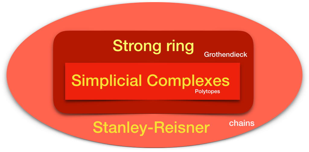
Simplicial complexes have a nice addition, the disjoint union. The empty complex is the zero element. One can extend this monoid to a commutative group in the usual way. (It was Grothendieck who formulated this in full generality, but we are all aware of this when extending natural numbers to integers or integers to fractions). The best way to encode the group algebraically is to represent simplicial complexes in the Stanley Reisner ring. The cyclic graph C₄ for example is xy+yz+zw+wx +x+y+z+w. Now, once one is in a ring, one can also look at -xy-x-y which is the negative of the complex xy+x+y. So, the mystery of what “negative complexes” are has disappeared. There is a problem however with the Stanley-Reisner picture. The full ring is too large. If we look at an element of the ring as a geometric object, then for most objects there is no cohomology, the unimodularity theorem does not hold etc. We have actually looked hard for algebraic constructs to prove the unimodularity theorem but the Stanley-Reisner ring is definitely too large. There is an other construct, the Zykov addition G + H of two complexes. It is the disjoint union as well as the set of all unions of sets in G and H. The Zykov addition is the discrete analogue of the join operation in topology. The join of two complete graphs is a complete bipartite graph for example. For examples see this paper. A graph has a nice duality operation in the form of the “complement graph”. The disjoint union addition is dual to the Zykov addition. One can also look at the complement of a simplicial complex, but unlike for graphs, where the complement is a graph, this is not the case for simplicial complexes any more. What about multiplication? I had searched for a multiplication compatible with the Zykov addition in January 2017 and found one. It turns out to be known as it is the dual to the Sabidussi strong multiplication of graphs. There is now a ring (which rules them all) of graphs which is really nice in that the Kuenneth formula holds for it. This means that the cohomology is compatible with the arithemetic. But there is more to it as the we can paint an other picture in which simplicial complexes are the basic ingredients. First of all, we can define a Cartesian product of simplicial complexes by looking at the product in the Stanley-Reisner ring. The problem with this is that the product is not a simplicial complex any more. But we can look at the ring generated by simplicial complexes within the Stanley Reisner ring. This ring is (as we have seen earlier) equivalent to the Strong ring. The strong ring really binds them all.

Particles and Space

Lets work now in the strong ring. It is a commutative ring in which the elements can be represented as concrete polynomials in the Stanley-Reisner ring. Simplicial complexes are special elements in this ring. We like this ring becuase unlike in the full Stanley-Reisner ring, the elements in the strong ring can be seen as geometric objects or “part of space”. We have also seen that when multiplying two elements, the spectra of the connection Laplacians multiply as the connection Laplacians tensor. We know this phenomenon when looking at the Fock space of particles which is used when doing “second quantization” at the hart of quantum field theory. A product of simplicial complexes behaves like a “multi particle state”, where the individual factors are the particles. Now, why don’t we just associate simplicial complexes in the strong ring as particles so that a general element in the ring (a space component) consists of a collection of multi particle states. Now, there is a beautiful theorem of Sabidussi which tells that the additive primes (the connected components in the strong ring) have a unique multiplicative prime factorization. This is the fundamental theorem of arithmetic in the strong ring! The strong ring is already more interesting additively as in the natural numbers, there is only one additive prime, the 1, while in the strong ring, every connected simplicial complex is an additive prime. But now, the Sabidussi theorem tells that while we have not a unique factorization domain (there are examples for which unique factorization fails), it does not fail for additive primes.

Simplicial complexes are the primes

Now, we have multiplicative primes, elements in the strong ring generated by simplicial complexes in the Stanley-Reisner ring. What are these primes? They are by definition elements in the ring which can not be written as G=H * K, with H and K both different from 1 (the complex with only one element). We have seen that on the connection graph level, there is a mirror ring of “graphs”, the Sabidussi ring, in which the multiplication is the strong multiplication. On simplicial complexes, the multiplication is the Cartesian multiplication which leads us outside the class of simplicial complexes (we have extended the class of simplicial complexes like that). Now, here comes the statement we originally wanted to include in this blog post (which got a bit longer than expected):

The multiplicative primes in the strong ring are the simplicial complexes.

Yes it is not difficult to show but it is by no means trivial. We have to prove that if we take two connected abstract simplicial complexes G and H and form the set theoretical Cartesian product G x H, then unless either G or H has only one element, the product is never a simplicial complex (otherwise we could have found a composite complex which is a simplicial complex). Now the product usually does not look like a simplicial complex but it could in principle be isomorphic to one. Since every product G x H contains the subcomplex K₂ x K₂ which has 3*3=9 elements, it is enough to show that K₂ x K₂ is not a simplicial complex. To see this, we first have to estimate how large the base set $V = \bigcup_A A$ can be on which a possible complex lives. As there are 9 sets, we see that |V| ≤ 5 as for a connected complex with base size n, the number of elements in the complex must be n+(n-1). Now we can just look at all the complexes which are possible on V with |V|=5 and see that none of them gives K₂ x K₂.

So, we have the following picture: the multiplicative primes in the strong ring are the simplicial complexes. They are the elementary particles in the ring. Every connected component in a ring (additive prime = particle) has a unique prime factorization into elementary particles. There are elements in the ring consisting of multiple disentangled particles which decompose in a non-unique way into elementary particles. As in the division algebra of Quaternions, where the prime factorization is a bit more complicated than in the integers, we have here a situation which is more complex but also like in the Quaternion case completely manageable.

Particle interaction

Non-uniqueness of prime factorization is always more exciting than uniqueness as it allows for particle exchange, interaction processes. Assume you take a single connected element in the ring, then it can be uniquely decomposed as a product of simplicial complexes. This is the Sabidussi theorem. Now combine the ring element with an other ring element. The unique prime factorisation now fails and the ring element can be decomposed as an other product of simplicial complexes. Now pick any of the new connected components (they are different from the previous ones), consider them as particles again. When meeting with an other connected component, they can be decomposed into elementary particles (simplicial complexes again).

Going from one prime factorization of a particle into an other prime factorization is a particle interaction process.

Connected space configurations (aka additive primes) can be seen as particles, indecomposable space configurations (aka multiplicative primes) can be seen as elementary particles. This is not the first allegory mixing terms of number theory with particle physics. See particle and primes. There is yet no reason to see why this should be relevant in physics. That statement would of course change if we could match pairs of non-unique prime factorizations with actual physical processes but that is definitely not yet the case. Still, it is intruiguing to see that mathematical theorems like the “quadratic reciprocity theorem” or the “Hurewitz-Frobenius theorem” or the “fundamental theorem of arithmetic for quaternions” (where uniqueness only happens modulo additional symmetry) or “Sabidussi unique factorization theorem” (where again uniqueness only happens under an additional topological assumption) can be interpreted in the language of particle physics. It is not completely useless as these theorems can be remembered better with some context: the Hurewitz-Frobenius theory of associative division algebras for example “explains” why the fundamental gauge groups are U(1), SU(2) and SU(3): also topology and arithmetic does its part as the only connected spheres in Euclidean space which are Lie groups are U(1) and SU(2). For SU(3) the allegory appears more like a stretch as a symmetry between the basic complex planes in the Quaternion division algebra but it appears less strange when seeing Lepton and Baryon structures appear combinatorically. It can be a Rubik’s cube type coincidence, but it makes the combinatorics of primes in Quaternions less look like something arbitrary. And vice versa, it makes the Standard model of particle physics less strange (when seen first, the standard model is anything else than divine …).

Physisics in general don’t like such analogies. The reason is that one has been burned too many times by “stupid associations”. The most prominent are the Kelvin knot vortex association. In a hundred years one might put the picture of particles as strings in the loony bin but in both cases, the dismissal misses an important point: Kelvin’s knot proposal spurred interest in knot theory, which is today an important part of topology. String theory has triggered a lot of interesting mathematics about topological invariants, symmetries, calculus of variations etc.
Mathematicians in general don’t like such analogies neither: the actually quite combinatorial paper dealing with equivalence relations of primes was bumped into physics. But there is interesting mathematics involved when looking at the strong ring:

The strong ring shows that the class of simplicial complexes can be extended naturally to a ring within the Stanley-Reisner ring and still have cohomology and spectral compatibility preserved. (For a topologist this is not surprising as the Grothendieck ring essentially does the same in topology, but there is a big difference: while the scalar Laplacian spectrum adds when taking Cartesian products, the connection Laplacian spectrum multiplies, as we have a tensor product of Laplacians than a Cartesian product). Also the Green functions g(x,y) defined by the inverse of the connection Laplacian L (which is defined for every ring element and not only for simplicial complexes) has still the property that the sum over all g(x,y) is the Euler characteristic. For every ring element one has cohomology, Euler-Poincaré, Hodge, McKean-Singer, Brouwer-Lefschetz as well as Gauss-Bonnet or Poincaré-Hopf results. One can even extend interaction cohomology to it, the cohomology which belongs to Wu characteristic similarly what simplicial cohomology does for Euler characteristic.

So, whether Space = Particles is a correct association is not that important. What is important is that we can now calculate with space and that the connection graph isomorphism allows us to do that all in graph theory within the Sabidussi ring rather than a rather opaque Grothendieck like ring. Calculating with graphs is VERY concrete. The addition is the disjoint union, the multiplication is taking the strong product. The complexity question how hard it is to distinguish primes or to factor a composite graph is completely open as it seems not even have been asked! The elementary particle interpretation of primes is for fun which makes the fundamental theorem of arithmetic for space more interesting.

[July 4: One should add that the characterisation of primes in the full Stanley-Reisner ring also could be interesting and that the primes in the subring generated by simplicial complexes might actually factor in the larger ring. Similarly, the ring of connection Laplacians of the ring generated by simplicial complexes is only a subring of the full Sabidussi ring of graphs. Indeed, all the Fredholm Laplacians have determinant 1 and most graphs don’t have this property. Also here it would be interesting to know whether one can decompose a “prime connection Laplacian” (coming from a simplicial complex) into Sabidussi primes.]