Graph limits with Mass Gap - Quantum Calculus

The graph limit

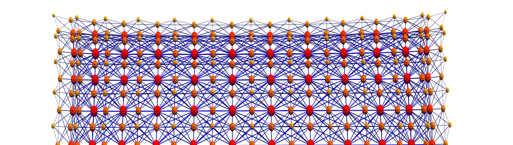
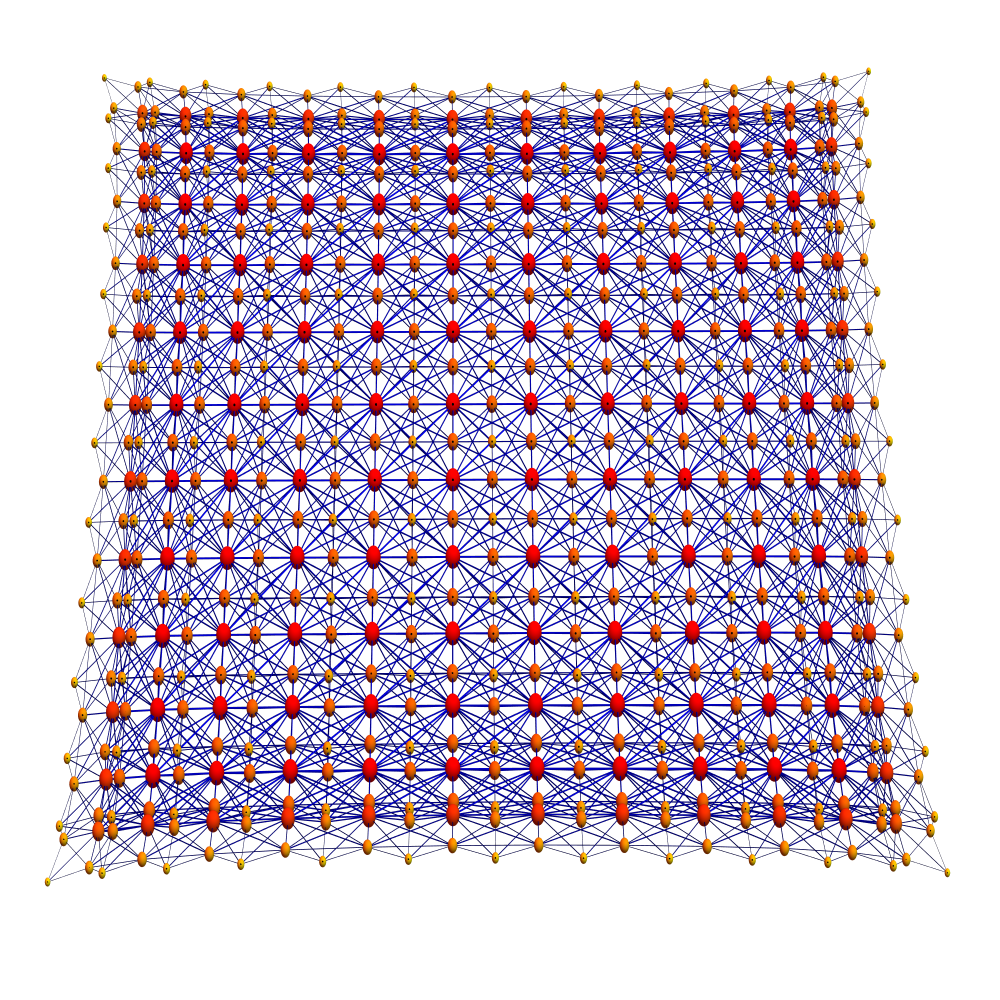
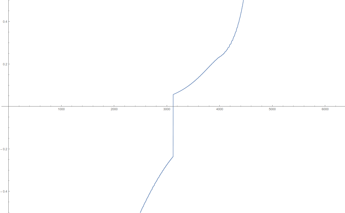
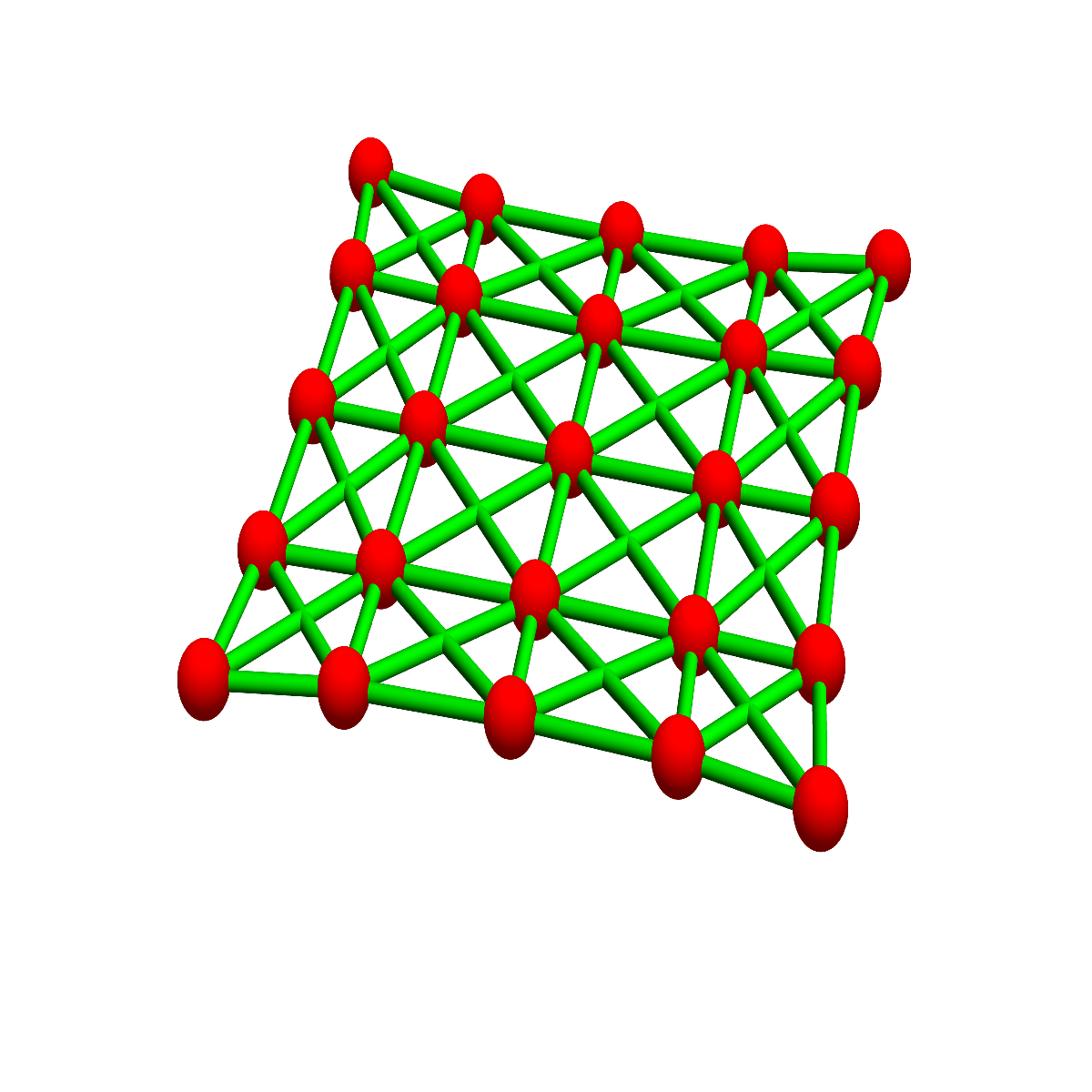
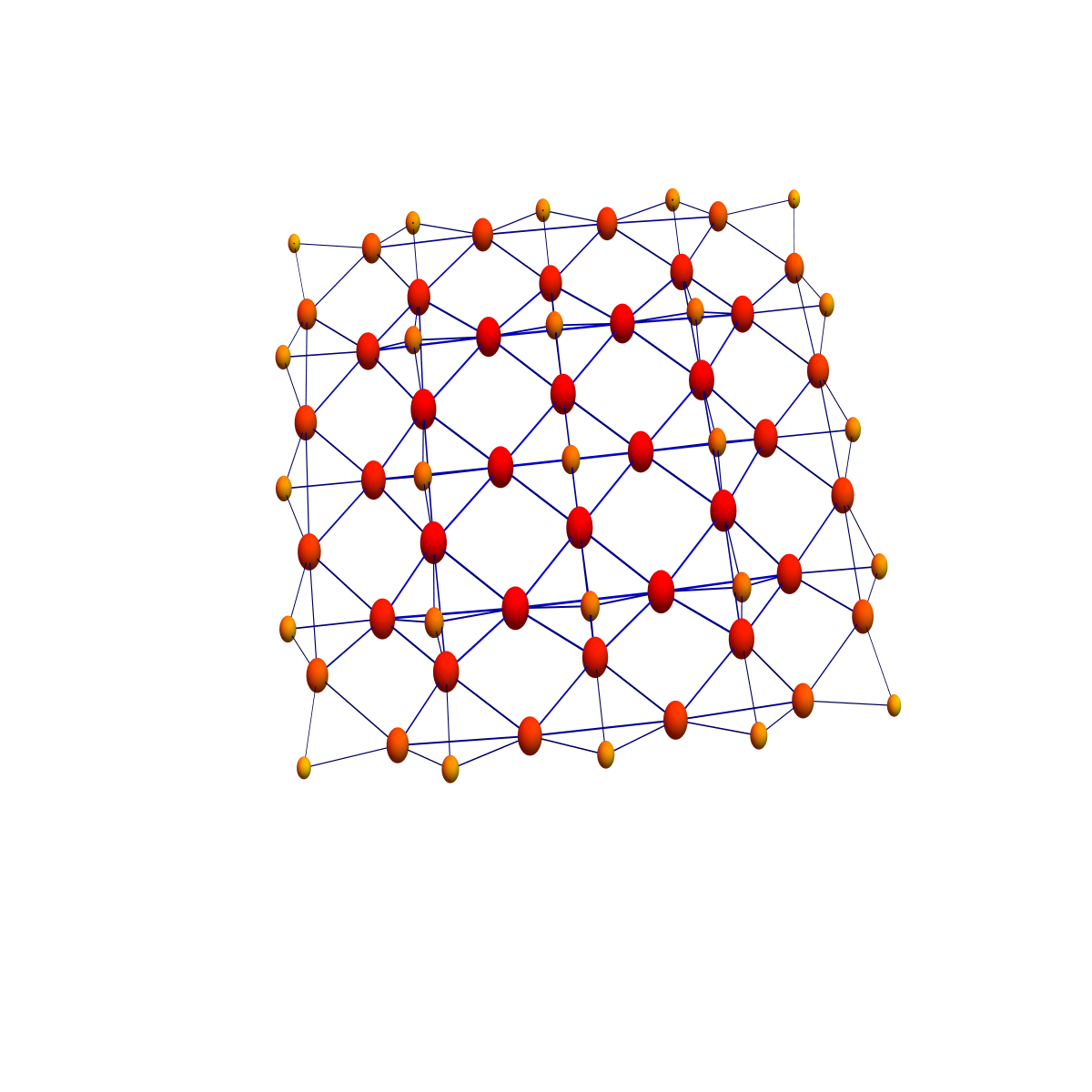
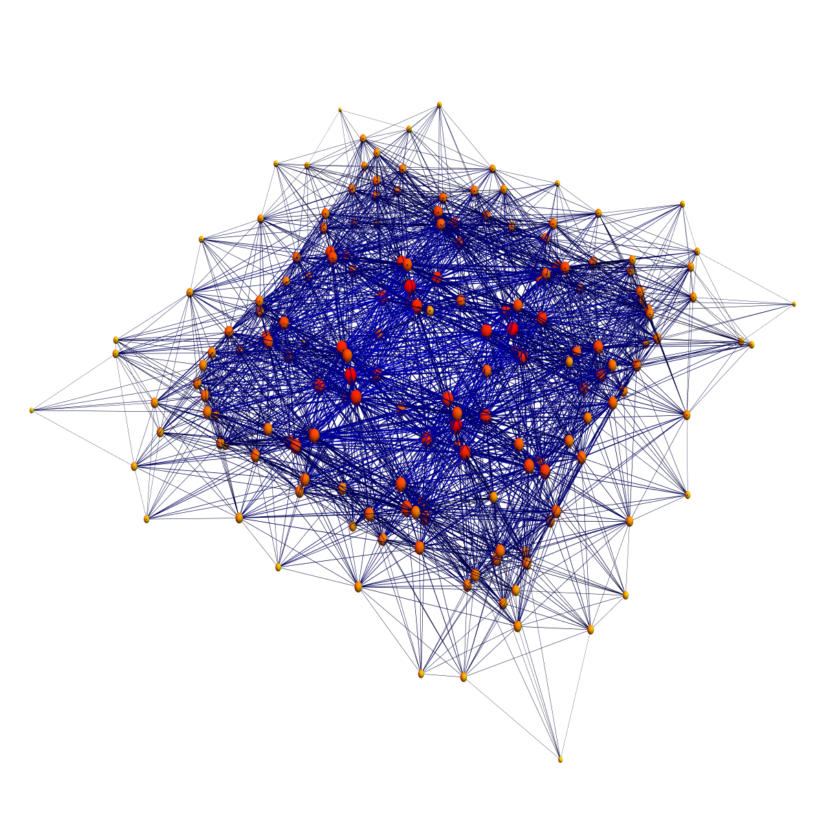
We can prove now that the graph limit of the connection graph of L_n x L_n which is the strong product of L_n‘ with itself has a mass gap in the limit n to infinity. The picture below shows this product graph for n=13, and to the right s part of the spectrum near 0 for n=40. We see the gap clearly. The spectrum avoids [-1/25,1/25]. The reason is very simple: the spectrum is the product of the connection graphs of L_n for which we know a spectral gap containing [-1/5,1/5].

Of course, the same argument goes in higher dimension and also for any initial graph G which is one dimensional, when taking the connection graph of $G \times G \times \cdots \times G$ . In some sense we have models of Euclidean space in arbitrary dimension for which the inverse of the connection Laplacian remains bounded even in a van Hove (infinite volume) limit. This is a different situation then what is the subject in statistical mechanics, where one looks at infinite particle limits (the original paper of Leon Van Hove from 1949). A biography of van Hove is here.

Why is this remarkable? Having an invertible Hamiltonian in a thermodynamic limit is nice, especially if the inverse operator g leads to a finite potential energy g(x,y) between two parts of space so that the total energy, the sum over all g(x,y) is the Euler characteristic.

But lets try to motivate why the connection graph is natural. It looks a bit strange at first as in two dimensions already the connection Laplacian of L_n x L_n has 3 dimensional parts. But it is not so strange if we look at how one looks at lattices in popular and familiar situations like lattice gas models or cellular automata.

Taxi and Uniform Metric

When dealing with the lattice Zⁿ, one usually does not pick the taxi metric l¹, where the distance is d(x,0)=|x₁|+|x₂|+…+|x_n| but the uniform metric l^∞ metric d(x,0)=max (|x₁|, ….,|x_n|) which is dual to the taxi metric. When playing the game of life cellular automaton for example, it is a game with the uniform metric: every cell has 8 neighbors. Also for lattice models in statistical mechanics like the Ising model, one can take either the l¹ metric or l^∞ metric so that |x_k| ≤ 1 is the unit ball of a site. In that model, one assigns a spin value $\sigma(x) \in \{-1,1\}$ to every lattice point and defines the energy $H_r(\sigma)$ = $-\sum_{x \sim y \in B_r} \sigma(x) \sigma(y)$ , where the sum ranges over all connected vertices in a ball $B_r = \{ |x|_{p} \leq r$ and studies functional integrals like $\langle f \rangle$ = $E[e^{-\beta H(\sigma)} f(\sigma)]/Z$ with $Z=E[ e^{-\beta H(\sigma)} ]$ . (The Ising model usually takes the l¹ metric.)

In the l^∞ metric has unit spheres which contain triangles (3 points all connected to each other in distance 1) while the l¹ metric, where in the unit sphere contains only 4 disconnected points, there is no edge. Both graphs miss the property of being two dimensional, but the 8 neighbor sphere has more friends: Most nearest neighbor automata take the uniform metric with 8 neighbors. But the other one is also popular, like in Ising or in numerical schemes or tightbinding approximations. In the weak coupling case l¹ , the Laplacian is replaced with u(x+1,y)+u(x-1,y)+u(x,y+1)+u(x,y-1)-4 u(x,y) which corresponds to the filter

| 0  1   0 |
| 1  -4  1 |
| 0  1   0 |

But also stronger filters using the l^∞ neighborhood are used, like in

| 1/4 1/2 1/4 |
| 1/2 -3  1/2 |
| 1/4 1/2 1/4 |

where the unit sphere has 8 members (containing triangles).

Discretisations

A discretisation of a metric d on Rⁿ is a countable subset V of R^d which is periodic (translational invariant with respect to n linearly independent translations) equipped with a graph structure G=(V,E) such that the geodesic distance in the graph is the same than the d-distance in R^d. The self-dual Euclidean l² metric d(x,0)=|x₁|²+|x₂ ²+ … +|x_n|² is the most symmetric, coming from an inner product, but it does not admit a discretisation which is a product lattice. The extreme Banach space metrics l¹ and l^∞ however both do.

The l¹ metric defines the weak Zⁿ lattice in which the unit sphere is zero dimensional.

The l^∞ metric defines the strong Zⁿ lattice in which the unit sphere is two dimensional.

Squares and Triangles

In two dimensions, there is a triangular lattice in which the unit sphere is one dimensional. But this triangulation does not come from a product structure. The fact that the product structures need quite a bit of bending to become triangular is the basic difficulty in de Rham’s theorem which links de Rham cohomology (a calculus based product cohomology which is used everywhere in calculus when dealing with operators like curl and div) and simplicial cohomology, in which the basic building blocks are simplices. Cubes are not simplices and either need to be cut (which breaks symmetry) or then require some homotopy deformations. The construction of a chain homotopy was tricky as one can see when looking at the original papers of the masters like de Rham. The problem of bending a cube to a simplex also appears in an ergodic setup to show the equivalence of geometric cohomology and algebraic group cohomology generalizing a result of dePauw in the two dimensional case.

Why product structures?

Why do we like a product structure? Because it allows us to reduce the situation to lower dimensional cases. Its like writing a random variable as a sum of uncorrelated random variables or performing conditional expectations to get the dimensions down. It is a basic principle to build up things from smaller parts and then bootstrap from lower to higher dimensions. Sometimes, the product structure is not obvious. A differential operator for example exhibits a product structure only after a Fourier transform. As one can see often in mathematics, products structures are more familiar and easier to deal with, especially in calculus setups, where we like to use concepts like partial derivatives and commutativity results like Clairaut or Fubini, product structures are not directly compatible with triangulations. The first who really realized the product structure of space was Descartes. It was there, of course, but nobody saw it. It is the concept of coordinates which reveals the product structure of space. In differential geometry later one has in the 20th centuray tried hard to get rid of coordinates again and make geometry coordinate independent (as coordinates are always a bit artificial, relying on a basis for example). Still, in the mathematical frame work which replaces it, tensor calculus and so the product structure (present at least locally also in non-linear situations) remains. Manifolds are patched up Euclidean spaces. Even more complicated topological spaces are equiped with sheaves carrying algebraic structures.

From topology to homotopy

If one is interested in properties which are homotopy invariants like cohomology, we don’t care so much about topological notions like dimension and can also allow discretizations of 2-dimensional space in which the unit spheres are not one-dimensional. This happens both for the weak lattice and the strong lattice. In the weak lattice, the dimension of the unit spheres have too low dimension, in the case of the strong lattice, the dimension of the unit spheres have too large dimension. But there is a difference in that the strong lattice behaves better for things which only depend on homotopy.

The weak lattice is not contractible in dimensions larger than 1. It has lots of holes.

The strong lattice is contractible in dimensions larger than 1. It is homotopic to a triangulation of space.

Product structure

Both metrics, the l¹ as well as the l^∞ metric come from a product structure. In one dimension, where all the l^p norms are the same d(x,y)=|x-y|, set V=Z is the only possible discretisation. Two integers (a,b) are connected by an edge if their distance is 1. Here is an observation:

The graph defined by the l¹ metric is the weak graph product of Z with Z.

The graph defined by the l^∞ metric is the strong graph product of Z with Z.

Connection Laplacians

The connection Laplacians of these two products look a bit more messy. The vertices are the simplices in the graphs above and two such simplices are connected, if they intersect. Already to the left, in the weak case, as 4 edges intersect, there are 4-simplices present in the connection graph. In the strong case, the dimensions are even higher, at least 7 dimensional.

The structure of space looks now more complicated because we display not only the zero dimensional and one dimensional parts as usual when drawing graphs but because we display also the higher dimensional structures: every simplex in the previous graph has become a vertex now. The connection graphs contain the Barycentric refinement graphs, which has the same vertices but where two vertices are connected only if one is contained in the other. In the connection graph case, we connect two vertices if they intersect.

Spectral properties

The product structure might look similar but it produces a spectacular different behavior on the spectral level. But we have to look at different Laplacians. In the weak case we have to look at the adjacency matrix to get spectral compatibility.

For weak products, the eigenvalues of the adjacency Laplacian add up.

For strong products, the eigenvalues of the Fredholm connection Laplacian multiply.

In the continuum, when taking the Cartesian product of manifolds, the eigenvalues of the standard Laplacian add up. In some sense,we get in the discrete strong product an entanglement which is not present in the continuum. It certainly also has to do with the choice of the Laplacian. Already in one dimensions, the connection Laplacian involves the adjacency matrix involving the simplices present in the graph.

The adjacency matrix or Fredholm adjacency matrix only addresses the zero and one-dimensional parts of space.

The Hodge or Fredholm connection Laplacian addresses also higher dimensional aspects of space.

In the Hodge or connection case, we look at all the simplices of a graph. It is interesting that this “looking at higher dimensional ingredients of space” will lead to entanglement in the sense that the energies don’t add up but multiply. Its like in a Fock space of quantum mechanics, where energies of independent particles add up, but that for multiparticle systems, the eigenvalues multiply.

Eigenvalues

One can explore this algebraically as one can see the lattice Z as a graph limit of a linear graph L_n or a cyclic graph C_n. There is a big difference between the two lattices. Lets define the sum-product of to numbers as xy+x+y:

For weak products, the eigenvalues of the adjacency matrices add.

For tensor products, the eigenvalues of the adjacency matrices multiply.

For strong products, the eigenvalues of the adjacency matrices are the sum-product of
the adjacency matrices.

The identity $(\lambda+1) (\mu + 1) = \lambda \mu + \lambda + \mu +1$ shows now why the eigenvalues of the Fredholm adjacency matrix L=(1+A) multiply. As we have seen that the connection graph functor G -> G’ satisfies (G x H)’ = G’ * H’, where * is the strong product the eigenvalues of the connection Laplacian multiply when we take a product. So far, there is little new, but we can exploit this now for a graph limit in higher dimensions.

Mass gap in a graph limit

By the central limit theorem for Barycentric refinements, the graph limit of a Barycentric limit of a graph converges universally depending only on the dimension of the initial graph. (See the article and some slides). As indicated already here, the situation becomes interesting if one takes connection Laplacians. In that case, there is a mass gap in the limit, the reason being that the limiting operator remains invertible.

This goes over to higher dimensional situations. We just have to take the strong product of the connection Laplacians to deal with connection Laplacians of products.

To summarize, we have models of space with a Laplacian which has also in the infinite volume limit a bounded inverse. We are not in a quantum field theory setup, but the interpretation is that the mass of the lightest particle is positive. In some sense, there is no infrared divergence. While we are at mentioning physics jargon, one could associate the Green function g(x,y) with a S matrix for space. Formally, we can write (1+A)^-1 = 1-A+A^2-A^3…. involving the adjacency matrix A. The sum on the right hand side is only defined by analytic continuation of function (1-s A)^-1 where the sum converges for small s. The boundedness of the Green function in the limit is remarkable. Actually, we know that the limiting operator is an almost periodic operator on a compact topological group. In one dimensions, it is the group of dyadic integers, in the n dimensional case it is the n’th product of these groups. Going to the product structure and refining each dimension sepearately allowed to bypass dealing with the Barycentric limit in higher dimensions, in which case, we still don’t know what the structure of the limiting compact topological group is.

Still, we are in a mathematical setup and just make a statment about the limiting density of states of an infinite graph limit. We still need to get an explicit formula for the density of states in the connection graph case analogues to the Laplacian case, where the density of states was the equilibrium measure on a Julia set. With that explicit formula, one can then get the density of states in higher dimensions by convoluting the logaritmic version of it. The limiting operator then definitely has absolutely continuous spectrum and just one gap.