If is a simplicial complex, and is a field, we have natural associated operators for which the matrix entries are locally defined as the energy of intersections of stable or unstable manifolds at x,y. See this document, where the set-up is also extended to non-commutative fields. As a physicist, one can think of as a complex valued wave function, for example, a solution of a Schroedinger equation. Now, we attach operators to a field, and in some sense produce operators from the field. This is a common theme in quantum fieled theory, which is the theory to quantize fields (hence the name). One can also think of it as a lattice gauge field, especially if one takes values in is a magnetic situation in 2D. I want look at this situation here and show some experiments about the density of states. It is already an interesting problem to investigate the spectra here. If is thought of as space or space time then one can think of this a lattice gauge field with the circle U(1) as a gauge group. The non-commutative setting was done in my latest paper so that one can also look at non-abelian gauge groups like , however, then the spectral theory needs still to be set-up more clearly there if one does not just want to write the matrices as real matrices with 4n entries. Lattice gauge theory (Wilson 74) had been popular, when I had been a grad student, but is currently belittled as a computer simpulated experiment which is (while rather condescending) actually a decent description, as what eventually counts in mathematics are theorems. And they are hard to come by in lattice gauge field theories especially in higher dimensions. So, the topic of lattice gauge fields is more like a numerical Monte Carlo scheme to compute things which would be hard to do in the continuum or to make sense of path integrals which in the continuum produce tremendous difficulties to make rigorous. For example, if G is the lattice and we put random valued fields at the oriented edges of the lattice, one can attach a magnetic flux” to each square cell (plaquette) by taking the product of the field values around the boundary of that plaquette. This is also called a Wilson loop. This produces a random field on the two-dimensional square cells (The lattice can be made into a 2-dimensioanl CW complex structure in which there are two dimensional cells which are not simplices.) One can then look at the corresponding magnetic operator I investigated once the spectral properties of this operator here (section 6) (see also this HTML version). The magnetic operator H probably has no point measure. I had used the Wiener theorem in Harmonic analysis and a discretization trick which allowed to compute the Schroedinger time evolution by iterating a map (a really cool idea because differential equations are much harder to integrate than iterating maps) and have a dynamics which has qualitatively the same behavior. This allowed me in 1998 already (with modest computational effort) to estimate the Wiener average on a 1000×1000 lattice. The experiments indicated that this random magnetic Laplacian has no eigenvalues, but nobody has proven this. It is related to the almost Mathieu operator but is a two-dimensional model and not one-dimensional as the much more famous Almost Mathieu operator, iconized by the Hofstadter butterfly.
[ The later has rock star status in mathematics, of course due to Hofstadter’s book Goedel, Escher Bach, which I war-shipped when it came out (I had been a Hofstadter fan in high school and remained a fan since) also due to Gardner type Hofstadter’s columns in the Scientific American journals, which we had at home and which was at that time a bit the window to newer science. I mostly . So, the Almost Mathieu problem had been on the minds of countless many kids already before Mandelbrot has hit the road with his fractal geometry of nature, that wave which washed ashore when I was in college and was unavoidable because everybody started to program the Mandelbrot set on the early PCs and students were flashing around copies of Mandelbrot’s book under their arms.So, for me, it had been concrete things like Rubik Cube the Hofstadter butterfly, the Mandelbrot set or simple but yet unsolved problems in number theory which made mathematics attractive. Now, a few decades later, the number of open problems in spectral theory, in number theory and in dynamical systems have grown even more. Spectral theory itself is a huge topic where we are largely in the dark, especially with inverse problems: like which spectra can be realized in a given model and how many times.The spectral type problem for the magnetic operator on the lattice is probably my favorite spectral problem, just because it has no free parameter. And the question is simple: are there eigenvalues with probability 1 or not? This is a localization problem which has not been solved yet and the work of mathematicians like Avron, Simon, Jitomirskaya, Last, Avila or Damanik on the Almost Mathieu operator indicate that the magnetic operator case might be difficult. However one has to note that the random magnetic operator case is also close to the Anderson localization part because unless in almost Mathieu (constant magnetic field), the field is now random. This tilts to believe that there should be some localized states a la Anderson. I should mention that there is a lot of other interesting mathematics related. For example, the question whether for a given IID magnetic field on the plaquettes, whether there is a field distribution on the edges which produces this IID field is a subtle cohomological problem in higher dimensions. My second paper on the subject and this paper on the cohomology of discrete Abelian group actions had a harder time even-so, I still think today that there are nice results there. For the magnetic operator for example, where IID fields on the edges can produce correlations on the plaquettes, the theorem of Depauw shows that one can realize the magnetic field through the vector potential on the edges. My paper from 2000 generalizes this to arbitrary dimensions. In dimensions 2 or higher, there is no ergodic cohomological restriction any more (the reason is a theorem of Feldman and Moore for a different related cohomology). This higher dimensional freedom is surprising if one knows that in dimension 1, where there are many field, which are not realizable gradients if is an ergodic automorphism. In two dimensions the question is whether for every field h on the plaguettes (2 form) there is a field k on the edges (1 form) such that h=dk.. I got into this topic because of dynamical systems theory and because this cohomology is essential also when trying to understand Lyapunov exponents. The later was an problem I was obsessed with as an undergraduate (thesis), graduate student (PhD thesis) and part of my postdoc time until reality hits and one has to worry about having bread on the table. I had been really lucky. Most mathematicians can pursue their problem of choice for a few years only and then are cut off. This is one of the mechanisms which has led to the myth that mathematics is a young persons game. The main reason of course is that most have no possibility to do math when they are older. There is a trial period in which one has to get great results. If that fails, the game is over. So, there is a whole army of young people working on the shoulders of giants for a couple of years, some making great results and fueling the myth that math can only be done by the young. ]
The Hofstadter butterfy from my page mathematik.com, posted there in 2005. I think this is still one of the best pictures of the butterfly. (It actually sows the Lyapunov exponent as a function of the energy and the magnetic flux parameter alpha.) As usual, one computes this by using periodic operators for which the spectrum is absolutely continuous located on a sequence of intervals. Understanding the periodic case and using periodic continued fraction expansion approximations in the general case allows to make mathematical statements about the butterfly like that it has zero Lebesgue measure (a result of Last). The first picture of this object has been done by Hofstadter and appears in his book Godel Escher Bach. Hofstadter had been interested in it due to self similarlity and self-similarity or self-reference is one of the central themes in this book and appears in logic (Goedel), visual art (Escher) as well as music (Bach).
Connection Laplacians
Now, after this rather lengthy introduction which explains a bit my interest in this and why it is natural for me to look at circle valued fields on a geometry, lets look at the operators L and g defined by a simplicial complex G and a random circle-valued field attached to it.
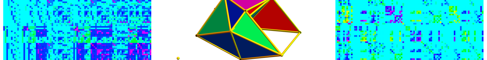
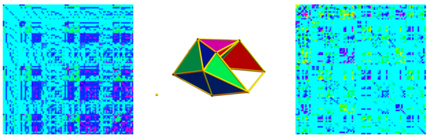
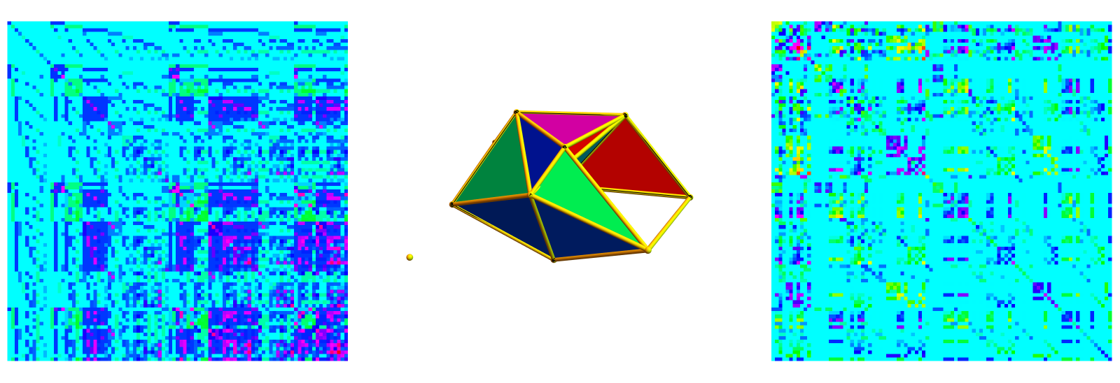
The matrix g, the complex G and the matrix L. In this case we have taken an Erdoes Renyi graph of the size 12 leading to a complex with 95 simplices and f-vector (12,33,35,14,1). The absolute values of the eigenvalues in this case are between 0.03889 and 52.5514. The matrix L has a maximal entry 6.05 in this case and g has a maximal entry 7.58. Whatever complex G we take, we end up with a density of states problem concerning the radial distribution of the eigenvalues.
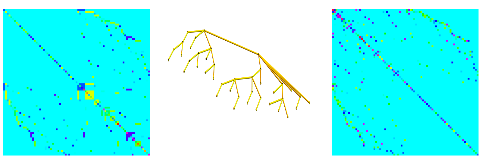
A tree with 41 vertices and 40 edges. Again, we see the connection Laplacian L and the Green matrix (the inverse of L). Again one can ask what happens with the spectrum for a typical field attached to vertices and edges of the graph.
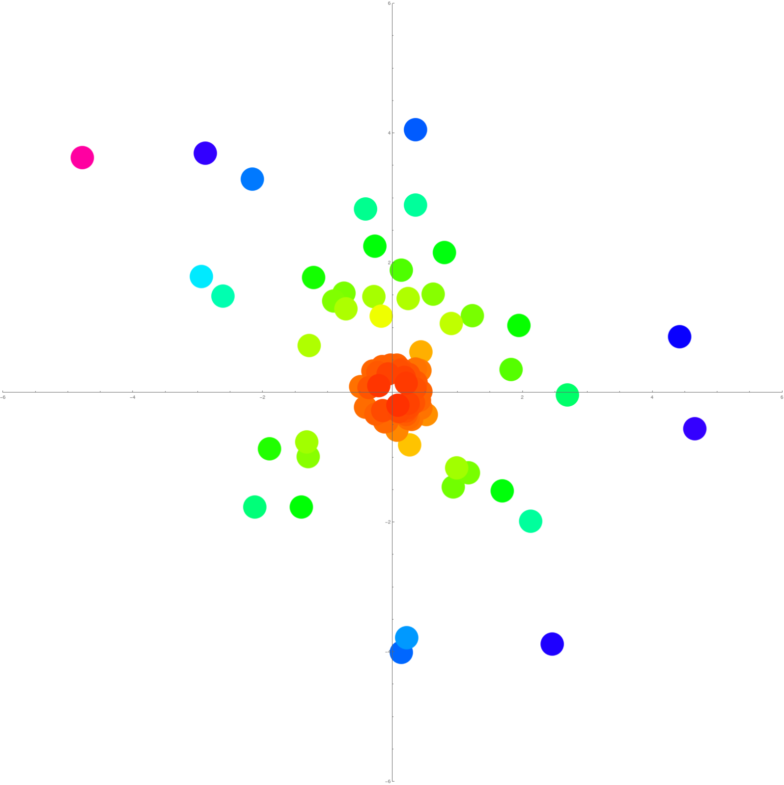
The spectrum in the complex plane for the above situation. This is a single experiment in the probability space of all configurations, which is the 81 dimensional torus, the probability space of all circle valued fields on this tree. (The Haar measure is the probability measure). What is the radial density of states distribution? We only know that the density of states is rotationally symmetric because multiplying all field values with a constant multiplies the operator with that constant.
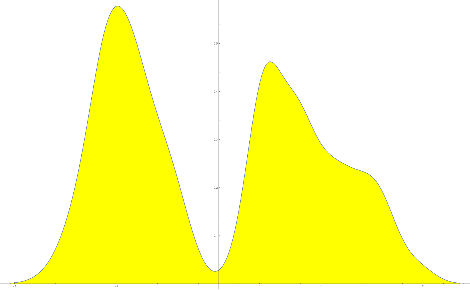
Radial distribution of the eigenvalues of a random field on the tree taken above. We see here the distribution in a logarithmic scale. There were 100 random field values taken. If we would take this tree and let it Barycentrically evolve, then the density of states approaches the universal case.
So, again, like for the magnetic Laplacian considered in the introduction, we again have models which only depend on the geometry and have no other free parameter. We actually do not need even the simplicial complex structure (the only axiom!) but can look at an arbitrary set of sets G. In this case we have proven that the determinant of the operators L and g are the product of all the field values and that L and are inverses of each other! This is amazing. If one looks at questions like mass-gap, Green function, difficulties with infinities when dealing with perturbation theory, it is just simply a relief to deal with operators which are always invertible. There is also quite a bit of physics related as the sum of the Green function entries is the total sum of the field values (this needs the simplicial complex structure however and does not hold necessarily for arbitrary sets of sets). Unlike for classical gauge field theories (vector bundles on manifolds for example), where the multiplicative group structure on the fibers is essential a priory, here the algebra structure matters (a commutative or non-commutative division ring is needed in order to define determinants). And now, even when the complex is infinite, there is a spectral gap, as long as there is a bound on the number of sets with which a given set can have connections. A mass gap is now almost trivially built into the system, hard implicit function theorems are not necessary and perturbation theory can be done with the standard implicit function theorem. Hard implicit function theorems are classically needed already in the one dimensional case when working on the lattice , like when looking at the Frenkel-Kantorova perturbation like of the free Hodge Laplacian which is the square of the Dirac operator with exterior derivative . Such perturbation problems are in general, on any manifold, difficult because for , the Hodge Laplacian is not invertible: there are always harmonic forms.
Universality
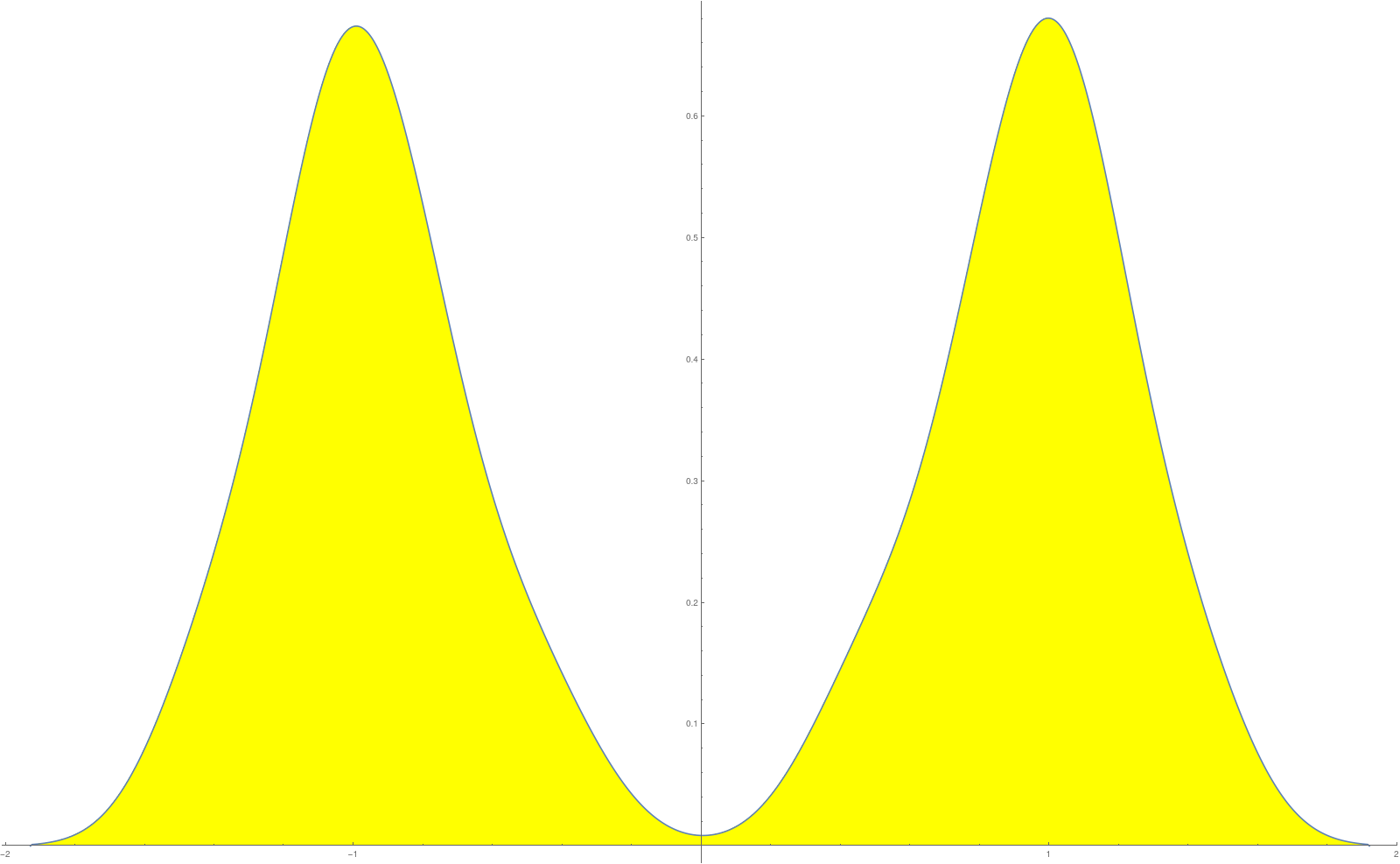
If we have a complex G, we can look at the Barycentric refinement of and iterate the refinement process and get a sequence of complexes . Now, the analysis shown for the Hodge or Kirchhoff Laplacian gives a universality. Also here, in the limit , there is a universal density of states which only depends on the dimension of G and not on G. In the one dimensional case, the distribution can be computed relatively easy for the Kirchhoff Laplacian. We have not yet done so in the case of circle valued random fields. The distribution of the appears in the one dimensional case to be symmetric but no more in dimension 2 or higher. Here is the picture if which already looks close to the limiting universal radial distribution one has in one dimensions. Why is the symmetry expected? If the field values are 1, then we have that spectral (symplectic type) symmetry for any complex. In one dimensions, there is more symmetry and is the Hodge Laplacian. I called this the hydrogen identity because the Hydrogen operator in quantum mechanics has this type of structure because the Newton potential 1/|r| is related to the Green function of the Laplacian in three dimensional space. There is still a lot to explore in the case of random circle valued fields also in van-Hove limits, where we have a provable spectral gap. The one dimensional case is special because under Barycentric refinements, this is the only dimension, where the vertex degree stays bounded.
The logarithmic radial spectral distribution for the cyclic complex with 40 elements. We took 100 field values and computed the eigenvalues then looked at the values of the logarithm of the absolute values. The explicit form of the density of states limit is certainly computable in this case as is the zeta function which we have computed in the topological case where the field value is .


=\psi(x)")

= \{ |z| = 1 \}")
")

")
 k^{-1}")


 = u(n+1)-2u(n) +u(n-1)")


|")

=\sigma(L^{-1}")

=(-1)^{dim(x)}") .
.