Tensor Products Everywhere - Quantum Calculus

Multiplicative spectrum

The energy theorem $\chi(G) = \sum_{x,y} g(x,y)$ holds for geometric objects in the Grothendieck ring X of cellular complexes: the connection Laplacian L of any ring element is unimodular and the Green function $g(x,y)=L^{-1}(x,y)$ is integer-valued. Since the ring product is close to the Cartesian product, it might surprise that the connection Laplacians is a tensor product of the individual connection Laplacians. But this has a nice effect: the spectra multiply: for any two $G,H$ in X, we have $\sigma(G \times H) = \sigma(G) \sigma(H)$ and $\sigma(G+H) = \sigma(G) \cup \sigma(H)$ . While the tensor product is not commutative, the product in X is. It is not a contradiction as the spectral theorem implies immediately that the connection Laplacians of $G \times H$ and $H \times G$ are similar essentially representing the same operator. It is nice to have not only the energy multiplicative, but also the spectrum multiplicative. It is not a surprise: spectral values of a Laplacian are measurable manifestation of energy.

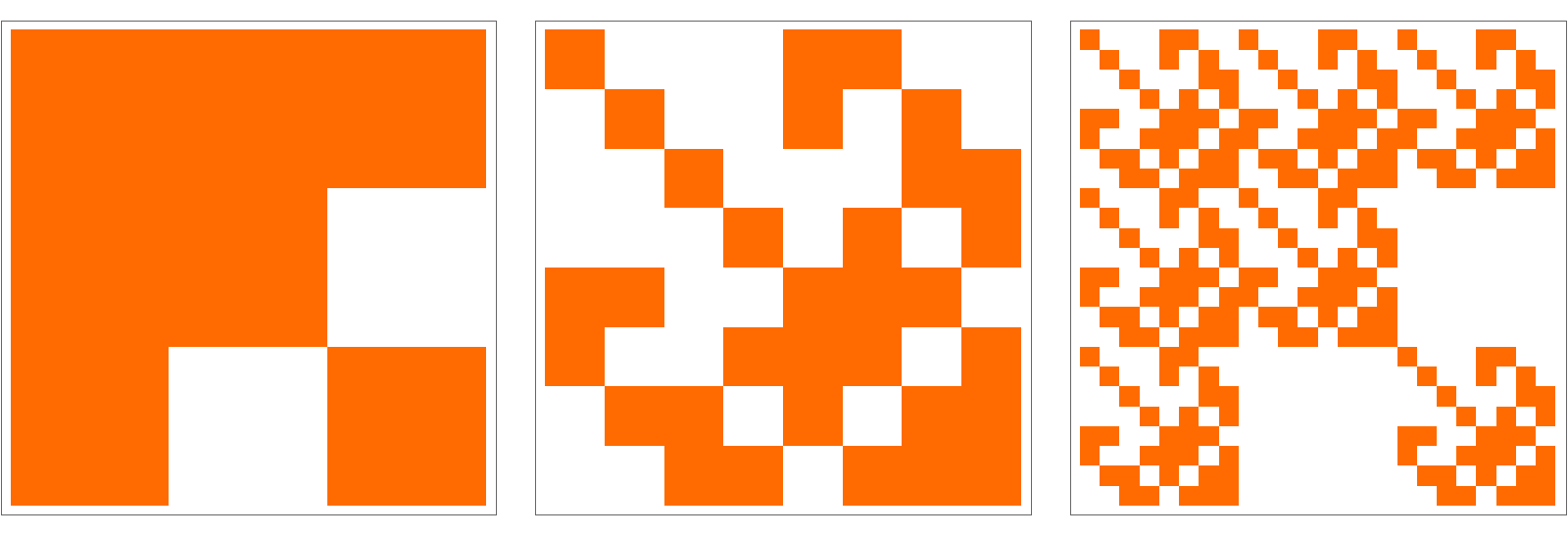
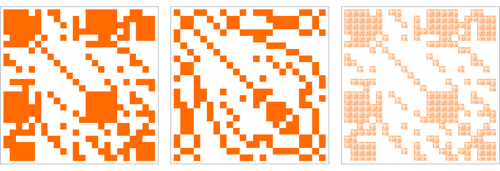
Here is an example. The first complex G is the Whitney complex of $K_2$ . It has 3 elements. The second complex is the Whitney complex of the circle $C_4$ . It has 8 elements. The product $G \times H$ in the Grothendieck ring has 24 elements. It is not the Whitney complex of a graph (it is not even a simplicial complex any more, but only a CW complex). But its connection graph $(G \times H)'$ is a graph and thats what we display in the next figure. In that graph, two elements (x,y) and (a,b) are connected if both (x,a) and (y,b) are connected in the connection graphs G; or H’ respectively. Note that this is not the tensor product of the connection graphs. The tensor product of G’ and H’ is a one dimensional graph with f-vector (24,48). The connection graph $(G \times H)'$ which we see here, has maximal dimension 5 and f-vector (24,100,156,120,48,8):

Now lets look at the connection Laplacians L and K of G and H. They encode the discrete CW complex and put a 1 if two cells intersect and 0 if not. The extremely remarkable fact that they are all unimodular had started that entire digression into connection Laplacians. Here they are. The color orange means 1, the color white means 0:

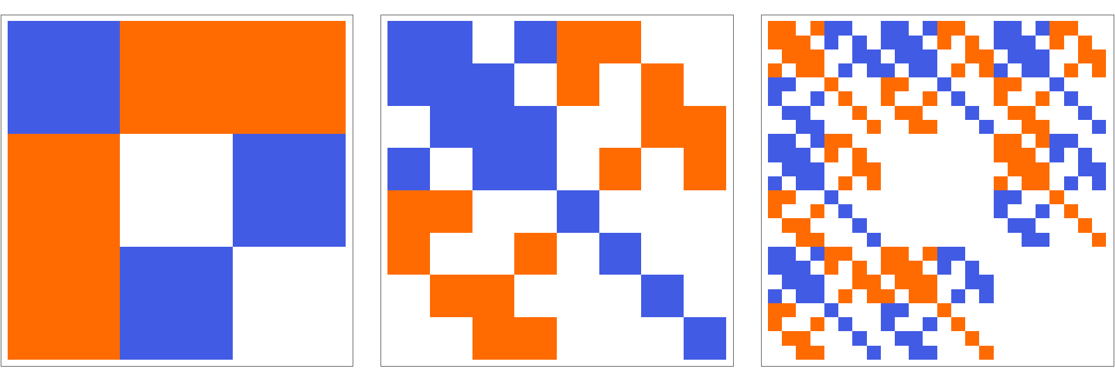
We see in the above graph the tensor product of L and K. The tensor product of K with L is a different matrix but its just that the basis is different in each of the two cases. The connection matrix construction can still be seen as a ring homomorphisms from the ring X to the tensor ring of symmetric matrices but this requires to identify isospectral selfadjoint matrices and so $L \otimes K$ and $K \otimes L$ .

The spectrum of the first matrix is $\{1+\sqrt{2},1,1-\sqrt{2}\}=\{2.41421, 1., -0.414214\}$ . The spectrum of the second is $\{2+\sqrt{5},1+\sqrt{2},1+\sqrt{2},-1,1,1-\sqrt{2},1-\sqrt{2},2-\sqrt{5} \}$ $=\{4.23607, 2.41421, 2.41421, -1., 1., -0.414, -0.414, -0.236\}$ . The spectrum of the third is the product: $\{10.22,5.82,5.82,4.23,-2.41,2.41,2.414,2.41,-1.75,-1,-1,-1,-1,-1,-1,1,-0.57,-0.41,-0.41,-0.41,0.41,-0.24,0.172,0.172,0.098 \}$ . Here are the Green functions, the inverse of the connection Laplacians just displayed. By the energy theorem, the total of entries are the Euler characteristic (which is 1 for G and 0 for H). Also the Green functions tensor: the tensor product of the Green function of G with the Green function of H is the Green function of $G \times H$ . In the following picture, the blue entries are places where the Green function value is -1. The networks are not complicated enough yet to feature any entries different from 0,1 or -1. We have seen that the diagonal entries g(x,x) are the indices 1-S(x) and in this case, all unit spheres S(x) still have either Euler characteristic 0,2 (spheres) or 1 (contractible). Also the super traces multiply as the super traces of the Green functions are the Euler characteristic too (this was the Gauss-Bonnet connection discovered in February and written down here.

In summary, the product of CW complexes behaves in a correct way: the product space has a natural potential energy theory, the right spectrum, the right Euler characteristic. It behaves naturally of what we expect from a physical product system even so there is no physical model placed in. There are no forces, no Lagrangians, no particles artificially placed in: it is geometry pure. Still, having a product allows now to do constructs done in field theory similarly as n-particle states are described by tensor products.

[Remark. The fact that the adjacency matrices of tensor products of graphs are tensor products (a well known fact) is now augmented with the fact that the Fredholm adjacency matrices of connection graphs tensor to the Fredholm adjacency matrix of the connection graph of the product. This is unrelated as the adjacency matrices and the tensor product deal with the category of simplicial complexes while the Grothendieck product is a construct which is only defined in the larger category of discrete CW complexes. Also, we have to stress that the product in the ring of networks (which is a product in the class of simplicial complexes or even in the class of graphs) is again a completely different product belonging to a completely different addition, the join operation. In the Grothendieck ring, the addition is the disjoint union.]

Tensor products !

Tensor products are defined for geometric objects as well as for maps between objects. The tensor product of linear spaces and matrices is a construct in multilinear algebra. It rarely appears in first exposures to linear algebra courses except maybe that we look at the concept of partitioned matrices. A $6 \times 6$ matrix for example can be seen as a $2 \times 2$ matrix of $3 \times 3$ matrices. Some of these matrices are tensor products. The tensor product of the operators is an operator on the tensor product of vector spaces. Unlike the Cartesian product of vector spaces which looks at all pairs $(x,y)$ and a basis $e_i + e_j$ , the tensor product of vector spaces takes pairs $(e_i \times e_j)$ as basis. The dimension of the Cartesian product of $R^n$ with $R^m$ is $R^{n+m}$ . The dimension of the tensor product of $R^n$ with $R^m$ is $R^{nm}$ . Tensor products can be defined more generally for modules and module homomorphisms.

Appearance in physics

In quantum mechanics, the tensor product of two Hamiltonians is the Hamiltonian of the two systems seen together. In the tensor product there are super positions possible which would not be possible in the case of the Cartesian product. There is hardly any algebraic construction which is described in so many different ways than tensor products. In physics it is an essential notion, as forces, fields, shears, curvature, metric or directional data are described by tensor fields. A basic construct is the Fock space constructed by Vladimir Fock.

Regaining linearity from multi-linearity

Mathematically, tensors are a construct which allow to describe multi linear constructs through linearity! This insight as well as much more is contained this handout of Keith Conrad. An example of this principle is the formula $p_k = tr(\wedge^k A)$ for the k’th coefficient of the characteristic polynomial of a matrix $A$ . While the trace is a linear operation giving the first coefficient the other coefficients depend in a multi-linear way on the coefficients of A. An example is the last coefficient, the determinant. Still, the exterior power (a Fermionic variant of the tensor product) allows to describe the determinant as something linear. Indeed, the determinant is the only n-linear Fermionic n-linear functional defined by a matrix.

Informal definitions

Tensors appear in all of mathematics and physics. There are now even youtube explanation which is brilliant but in the end, one still wonders “what is a tensor”? Some of the simplest tensors are vectors and matrices. Even there, the definitions can be confusing. One can still see today the poor definition “a vector is a quantity which has length and direction”. It is not only wrong (the zero vector is a vector which has no direction), but also so vague that it applies to a “motion picture”. A movie has a “direction” (the director) and a length (the number of minutes). This is not mathematical pedantry: the informal definition is not only wrong, it is also more complicated: a good working definition for affine vectors is that a vector $v=\vec{PQ}$ is defined by an ordered list of two points $P,Q$ in a linear space. One can then say that two vectors with the same components are “equal”. This allows to work in informal way with linear vectors too.

Tensor product of adjacency matrices

The tensor product of a $n \times n$ matrix $A$ and a $m \times m$ matrix $B$ is defined as the linear map on $R^n \otimes R^m = R^{n m}$ by $A \times B (e_k \otimes e_l) = A e_k \otimes A e_l$ . The tensor product $G \otimes H$ of two graphs $G=(V,E),H=(W,F)$ is defined as the graph for which the vertex list is the Cartesian product $V \times W$ and where $(a,b)$ is connected with $(c,d)$ if $(a,c)$ and $(b,d)$ are connected. The following is “well known”:

The tensor product $G \otimes H$ of two graphs G,H has an adjacency matrix which is the tensor product of the adjacency matrices of $G$ and $H$ .

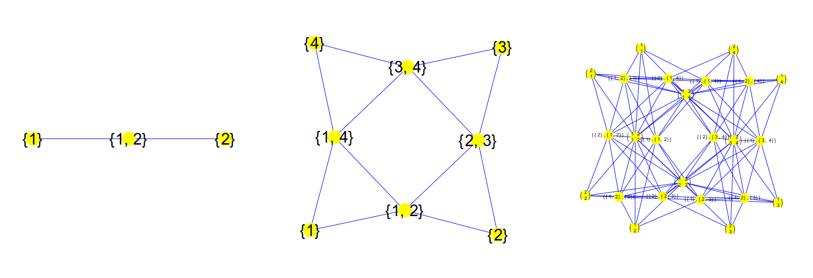
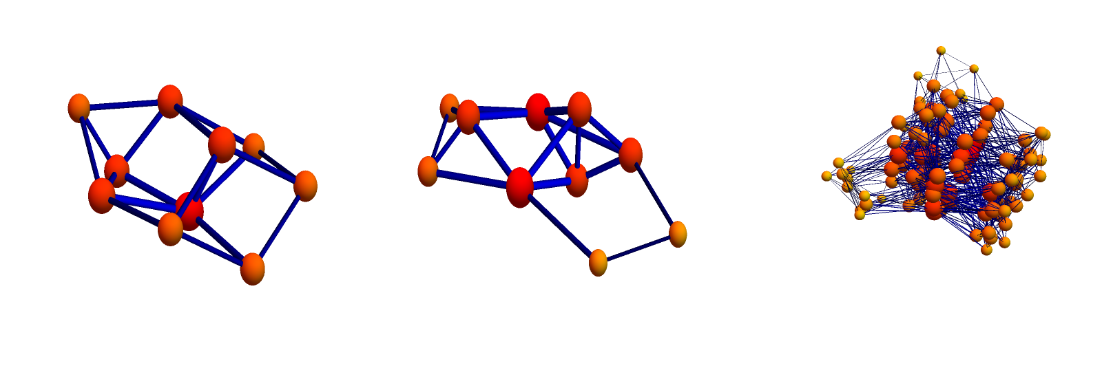
An example: first two graphs and their tensor product. Then the adjacency matrices:

Tensor product of connection graphs

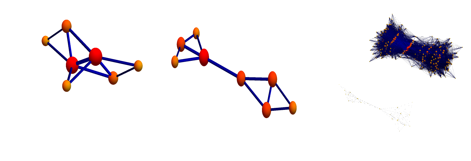
The Cartesian product of two discrete CW cellular complexes is defined in the class of CW cellular complexes. Its cells are the Cartesian product of the cells. Its Barycentric refinement is a cellular complex again, actually the Whitney complex of a graphs. This graph $G_1$ is given by the property that (a,b) is connected to (c,d) if both (a,c) and (b,d) are connected.

If $L'$ and $K'$ are the connection Laplacians of $G$ and $H$ , then the tensor product of $L'$ and $latx K’$ is the connection Laplacian of $G \times H$ . The Barycentric refinement of the Cartesian product of $L$ and $K$ is what we called $K \times L$ .

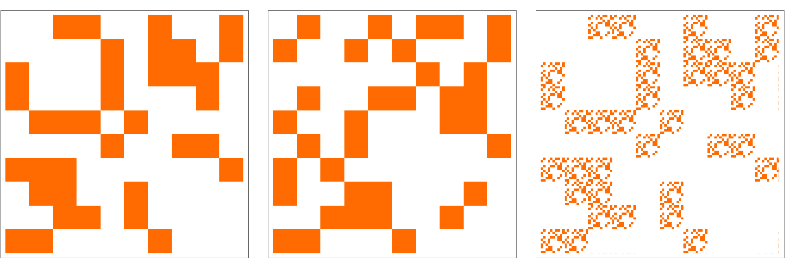
Here we see two graphs, the connection graph of the product complex, then the Fredholm matrices of the connection graphs of G,H and G x H:

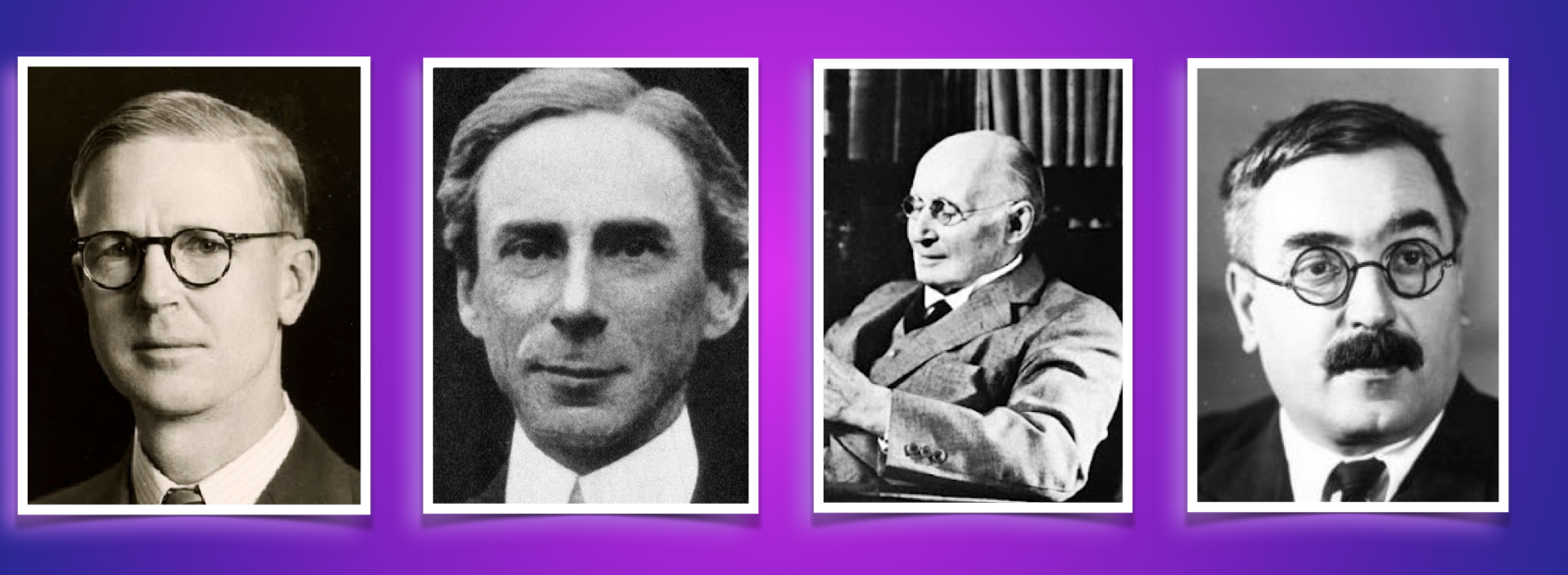
Some mathematicians

Here are some mathematicians associated to tensor product constructs. First Hassler Whitney (1907-1989) who also defined first the modern notion of manifold (1936). Whitney earned his PhD at Harvard in 1932 with work on graph coloring. He is commemorated in many mathematical constructs like the Whitney umbrella, the Whitney extension theorem, the Whitney embedding theorem. He seems have been the first to introduce the tensor product of modules in 1938. this book mentions that Murray and von Neumann had in 1936 invented a direct product of Hilbert spaces already. Then Bertrand Russell and Alfred North Whitehead, the authors of Principa Mathematica, which first seems to feature the tensor product of graphs 1912. I personally suspect that NOBODY has ever read and checked all of “Principia Mathematica” in detail. It is a monster. But I also suspect that in future, computers will be able to rewrite the and validate it. Finally, Vladimir Fock (1989 – 1974) who introduced the Fock space. As mentioned in this stack exchange, Bourbaki in 1948 cemented in the tensor product as a central object in multilinear algebra. The currently best write up on tensor product I can find is by Keith Conrad [PDF]. In that document, Gibbs is credited for the first construct 1884 who called it “indeterminante product” and Ricci in the 1880ies and 1890ies for introducing tensors to differential geometry. Still according to Conrad, Ricci and Levi-Civita referred to tensors by the name “systems”.