Discrete Hopf Theme

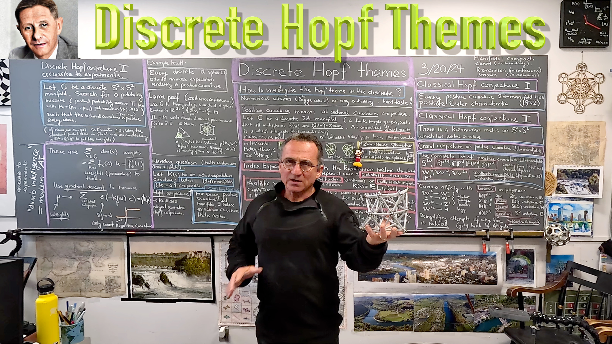
Here are three catchy open problems in differential geometry. As with any problem, we can look how to formulate discrete versions. The first problem is whether a positive curvature 2d manifold has positive Euler characteristic, the second is whether there is a positive curvature metric on and the third is whether the list of current positive curvature 2d manifolds is complete (). For the first problem, an idea is to exclude odd index critical points for Morse functions coming from a Nash embedding (take linear functions in the ambient space); the Morse inequalities would then imply that the odd Betti numbers are zero, which would imply positive Euler characteristic. For the second problem one needs a systematic search. For the third problem, one can look at situations with additional symmetry. There is a strange affinity between Bosons in the standard model and the list of positive curvature manifolds (2020). See this blog here. For the Grove and Searle theme one has to note that all currently known positive curvature manifolds admit a Lie group symmetry. In dimensions 6 and 8, one has with the additional symmetry assumption positive Euler characteristic. For positive curvature in the discrete defined by the cardinality of embedded wheel graphs alone, see the Mickey-Mouse Sphere theorem. [It was also featured in a talk about parameters (PDF) for communicating mathematics. I wanted especially to make the point there that abstraction is a bottle neck in communicating mathematics.] In a classical frame work, I tried once in the classical setting to find a curvature which is built from sectional curvatures and which is a deformation of the Gauss-Bonnet-Chern curvature. There is an integral theoretic approach to the entire Gauss-Bonnet theme. Just take a probability measure on Morse functions or vector fields or locally injective functions (in the discrete) to see Gauss-Bonnet as an expectation of Poincare-Hopf. This allows in principle to build a curvature on positive curvature manifolds which is positive. Nobody has found such a metric so far, but it has not been excluded. In dimension 6 and higher, the Gauss-Bonnet-Chern curvature can become negative somewhere. But this curvature is one of many. Especially in the discrete, we can conveniently search for probability weights. This is a fancy point of view, especially today, when everybody talks about large language models which are nothing else than such flexible structures in which weights allow for deformation. It is a big disappointment for AI researchers that such “dumb” AI is so successful. The math does not exceed undergraduate math but it can describe complex phenomena like Navier Stokes already better than the fancy PDE stuff. For me, having been working in 2003 (more than 20 years ago) on math chatbots, where we taught the bot by hand, this is such a big disappointment. Its like solving a beautiful math problem by brute force!

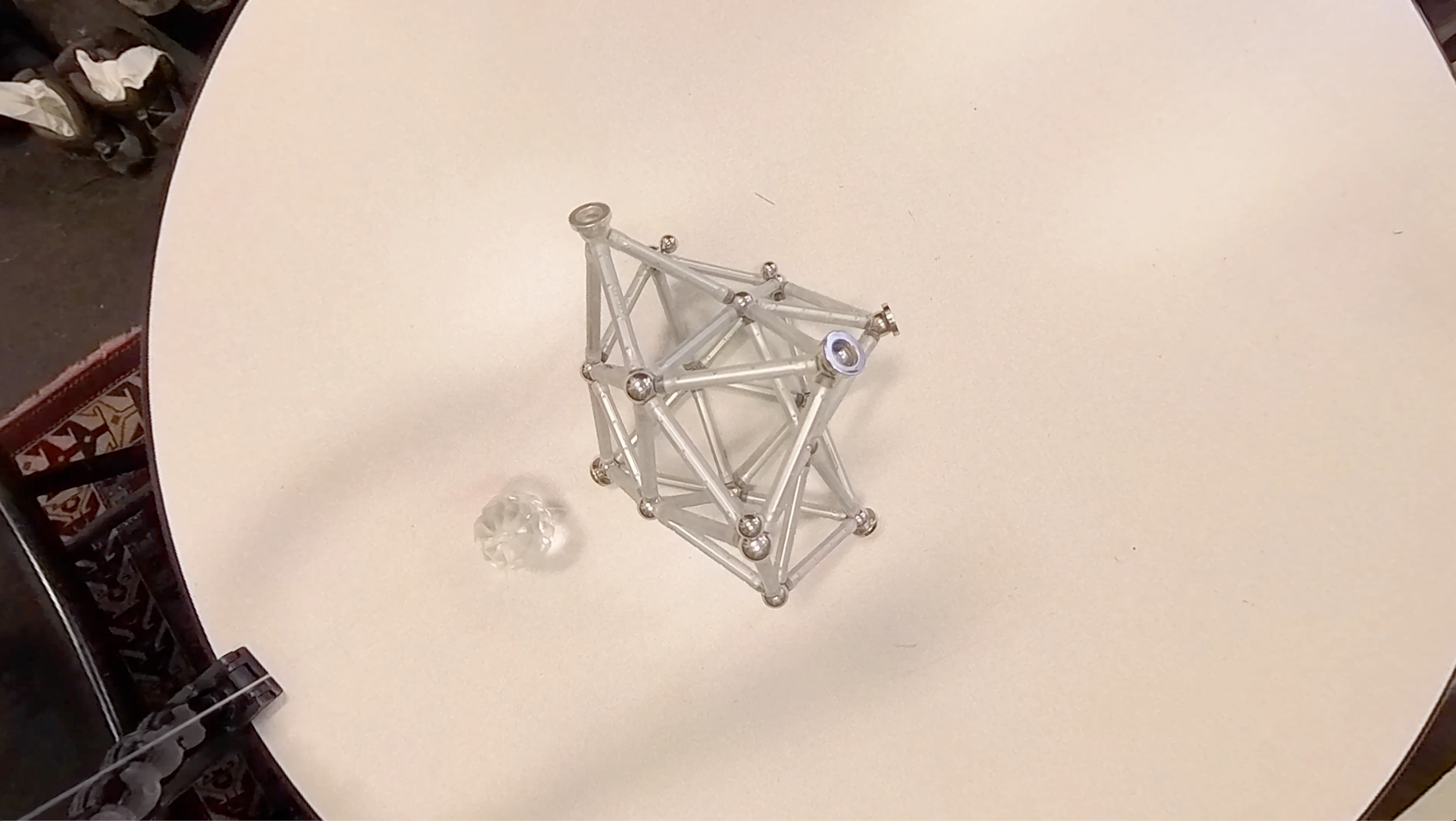
Update of April 22, 2024. I just made an experiment with a discrete projective plane G with f-vector (6,15,10). There are 31 simplices and 25 simplices allow tuning of the probability measures. There are 60 parameters to tune (with some constraints as we have probability measures, we use a soft max idea from machine learning). What one can do is write down are the explicit expressions for the curvatures in terms of these variables. In the picture we see the expressions. Adding up all these curvatures gives the Euler characteristic 1 by the Gauss-Bonnet theorem (which we talked about last week). One can do that symbolically using all the 60 variables. One can see the formulas for the curvatures to the right. Now, I did manually some graduate descent using a few dozen steps from a random initial condition of probabilities. The curvature now becomes positive in general. As the energy functional, I took the sum of the negative sigmoids of the curvatures which add up the negative part of the curvature and annihilate the positive parts. Minimizing this functional should produce positive curvature. The left picture below shows the curvature expressions in dependence of the variables. Filling in values for the X(k,l) (the l’th vertex in the simplex k) produces then numerical curvatures. But the expressions which are analytic in all variables can be differentiated. The gradient is nice (but complicated). If running the above code, it first produces the curvature expressions, then adds them up to get the Euler characteristic formally (which is the analog to compute the total curvature on a Riemannian manifold for an arbitrary Riemannian metric). Then a stupid gradient decent is used (not adapting the size, nor doing anything fancy. Sometimes we get to a positive curvature regime. This prototype computation demonstrates that one can in the discrete without any tensor calculus work in a differential geometric setting.

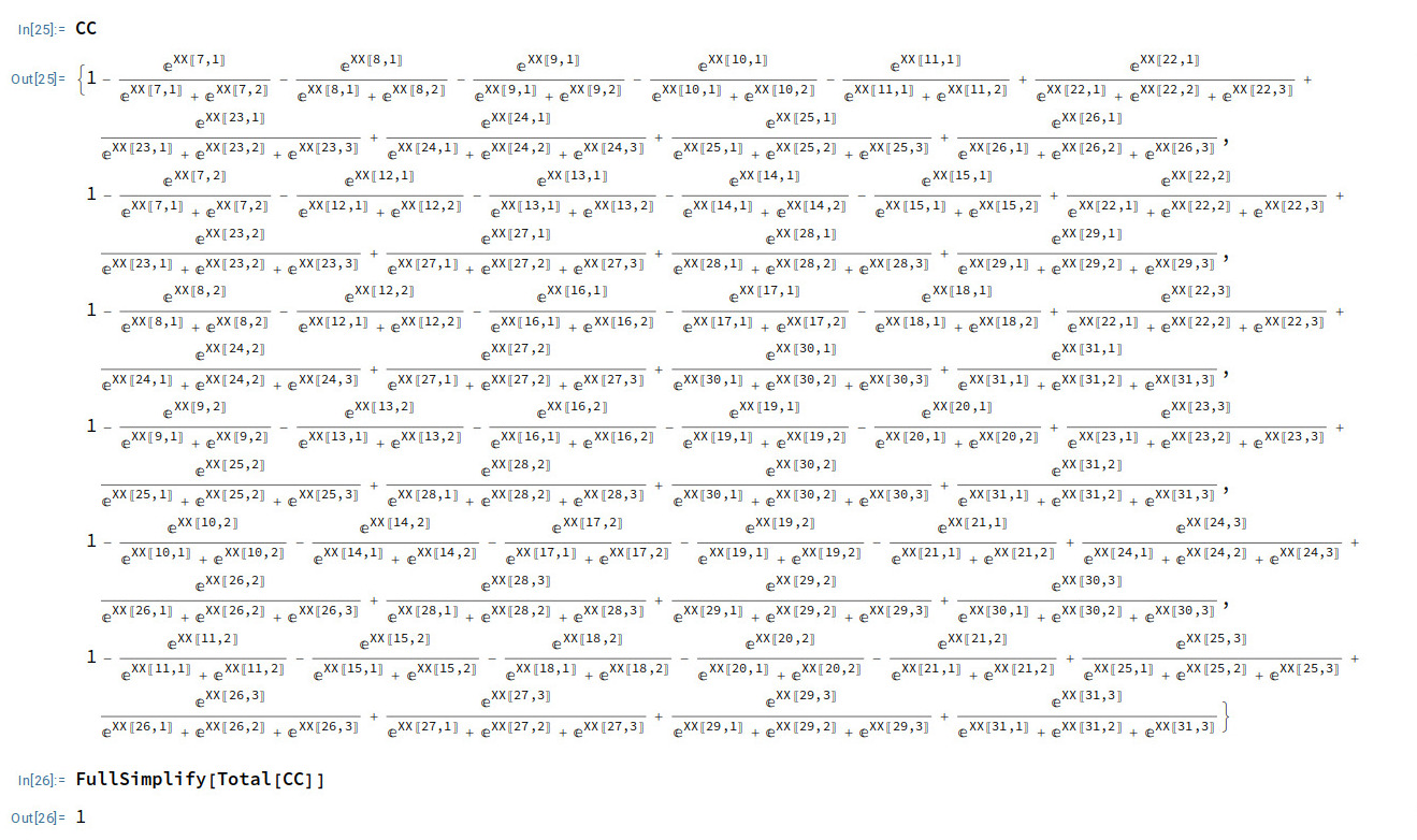
Here is the code which uses a gradient method in a 60 dimensional space of parameters to get to weights producing positive curvature. The geometry is a discrete 2 dimensional projective plane which initially has also negative curvature. We tune the parameters (Riemannian metric) to get to positive curvature. The code uses the general Gauss-Bonnet theorem which also works in general for delta sets:

G={{1},{2},{3},{4},{5},{6},{1,2},{1,3},{1,4},{1,5},{1,6},{2,3},{2,4},{2,5},{2,6},
{3,4},{3,5},{3,6},{4,5},{4,6},{5,6},{1,2,3},{1,2,4},{1,3,5},{1,4,6},{1,5,6}, {2,3,6},{2,4,5},{2,5,6},{3,4,5},{3,4,6}};

V=Union[Flatten[G]]; L=Length; W=Quiet[Table[Y=Table[Exp[x[[k,l]]],{l,L[G[[k]]]}]; 
   Y/Total[Y],{k,L[G]}]];
K[v_]:=Sum[g=G[[k]];q=W[[k]];If[MemberQ[g,v],
  l=Position[g,v][[1,1]];(-1)^(L[g]-1)*q[[l]],0],{k,L[G]}];
CC=Table[K[V[[k]]],{k,L[V]}];
FullSimplify[Total[CC]]   (* gives Euler characteristic 1 *)

sigma[t_]:=1/(1+Exp[30*t]); F = Total[Map[sigma,CC]];
X=Quiet[Flatten[Table[x[[k,l]],{k,L[G]},{l,L[G[[k]]]}]]];
grad=Table[D[F, X[[k]]], {k, L[X]}];
r=Table[Random[], {L[X]}];
Do[f0=Table[X[[k]]->r[[k]],{k,L[X]}];F0=F/.f0;
grad0=grad/.f0; r=r-0.01*grad0,{120}];
curvatures= CC /. f0
Total[curvatures]

The main topic in the video is the use of index expectation also for defining “positive sectional curvature”. For higher dimensional manifolds, we usually have lots of wheel graphs with negative curvature. The fluctuations of sectional curvature are big. One possibility is to take a discrete approximation of a two dimensional plane and take the average curvature there inside. But this is what one would call a “numerical approach” as there are lots of choices which one would have to make. Currently, I think the best definition of positive curvature in the discrete is that there is a probability measure on vector fields [remember, a vector field is just a map which assigns to a simplex a vertex within the simplex. When using this map to transport the energy from x to the vertices, one gets a Poincare-Hopf index which by definition satisfies Poincare-Hopf. If the assignment F(x) is the minimum of a locally injective function f on the vertices, one has the analog of a vector field]. A probability measure on vector fields is nothing else than attaching a probability measure on each simplex assigning to its points weights. This gives Gauss-Bonnet. The weights certainly also define now curvature for each embedded wheel graph (only the weights on edges and triangles obviously are involved there). A discrete manifold is now a positive curvature manifold if there are weights such that all wheel graphs have positive curvature. What happens with this definition is that it is simple and elegant and gives what one expects to happen. Imagine the discrete manifold embedded in an ambient manifold (we assume for a moment, for the sake of motivation to give in to the horror of using geometric realizations, we are after all in a quantum calculus blog where we do not accept anything involving limits and especially do not accept the continuum for granted). If G is embedded in M and M is isometrically Nash embedded in an ambient Euclidean space E, then we can use the probability measure from linear functions in E to define Morse functions on M and locally injective functions on G (all this happens with probability 1 of course, already Morse knew that in the Morse case). Now, if M has positive curvature, then, if G is a sufficiently fine approximation, then G has positive curvature in our sense. Our definition of positive curvature in the discrete is not only much more elegant than any tasteless numerical scheme but it is also more realistic.

[Update of April 25: the definition is still way too strong to be realistic: take the geometry and embed into it a 2-dimensional surface of higher genus. The Sard theme has shown how we can do that almost for free. Now, the 2 dimensional curvature on this surface must be negative at some place and no tuning of the parameters can save that (unless we would allow to use a curvature which does not satisfy Gauss-Bonnet but from my personal point of view, any curvature that does not satisfy Gauss-Bonnet is over rated. One can argue that the scalar curvature is important in relativity because it is the basis of the Hilbert functional for GR, one the other hand, one must really question whether this elegant variational problem is really the yellow of the egg. We all know that in the very small, GR and QM do not appear to be compatible. A quantied functional like Euler characteristic can make a lot of sense too, mainly of course because there are half a dozen of very important theorems in mathematics that deal directly with Euler characteristic or generalizations of it. By the way, for me it is always a bit silly to ask “why” a given structure appears in physics. Why does a fruit fly have green eyes? Well, it just so happened to turn out. What is much more interesting is what structures produce interesting theorems. This is what makes a structure interesting. The theorems should be beautiful, simple and still surprising. Whether nature has adapted a given structure is a great quest but we almost by definition will never be able to find out “why”. It could all be just projected to us in a simulation, and the kid playing the game in the meta world outside is again a simulation in an other simulation. Dozens of Sci Fi movies explore this theme. The 3-body problem show (the latest of this kind I have seen) allows the simulation to happen in a game VR headset or then directly by interacting in the brain. The “gods” in the 3-body system who want to immigrate to earth are there also able to hack the senses of the humans like seeing the universe flicker, or see numbers counting down to a dooms day etc etc. How can we ever prove that there is not such a mechanism hacking us, or even our mathematical thinking? Despite all this, when I would be asked what happens really, I would think that all these meta thinking is very unlikely, so unlikely that it does not happen and that mathematical structures are natural and inevitable also without any intelligence observing them and that that they exist to serve some purpose, which we might never know to see. But for a mathematician, there would be a much easier “solution” to the entire ontology problem: just look at the empty world, with nothing in it, no space, no time, no mass, no structure. It is the most elegant problem but rather nihilistic. What did Walter say in the Lebowski movie: see it yourself. ]

By the way, when mentioning integral geometry in the context of Riemannian geometry, one should always bear in mind that the interest in integral geometry exploded in differential geometry, with Blaschke, the (academic) father of Chern as well as Herman Weyl, who used tube methods for accessing differential geometric properties. Having a probability measure on Morse functions classically of course by the Crofton formula defines a metric so that giving a probability measure on Morse functions already classically can replace tensor field definitions. It also in the discrete would provide us with a metric on the graph, meaning assigning distances between nodes.

Heinz Hopf (1894-1971) had an immense influence at ETH Zuerich. Half of my teachers at the poly and also my high school math teacher were all Hopf descendents: direct (kids of Hopf) Urs Stammbach (algebra I and II), Ernst Specker (ffirst yearlinear algebra I and II andlogic). Then the academic grand kids: Roland Staerk (my high school math teacher), Christian Blatter (Banach algebras), Max Jeger (classical geometry and differential geometry), Max-Albert Knus (commutative algebras) Guido Mislin (classical groups), Hans Laeuchli (first year calculus I,II, non-standard analysis and model theory), Erwin Engeler (set theoretical topology, math software and computation) and Peter Henrici a student of Eduard Stiefel who was a Hopf kid (numerical analysis) and Peter Laeuchli (also a Stiefel student) (programming and numerical analysis). Hopf had taste which inluceed to ask good questions. Hopf can be read today still. See his math genealogy site.

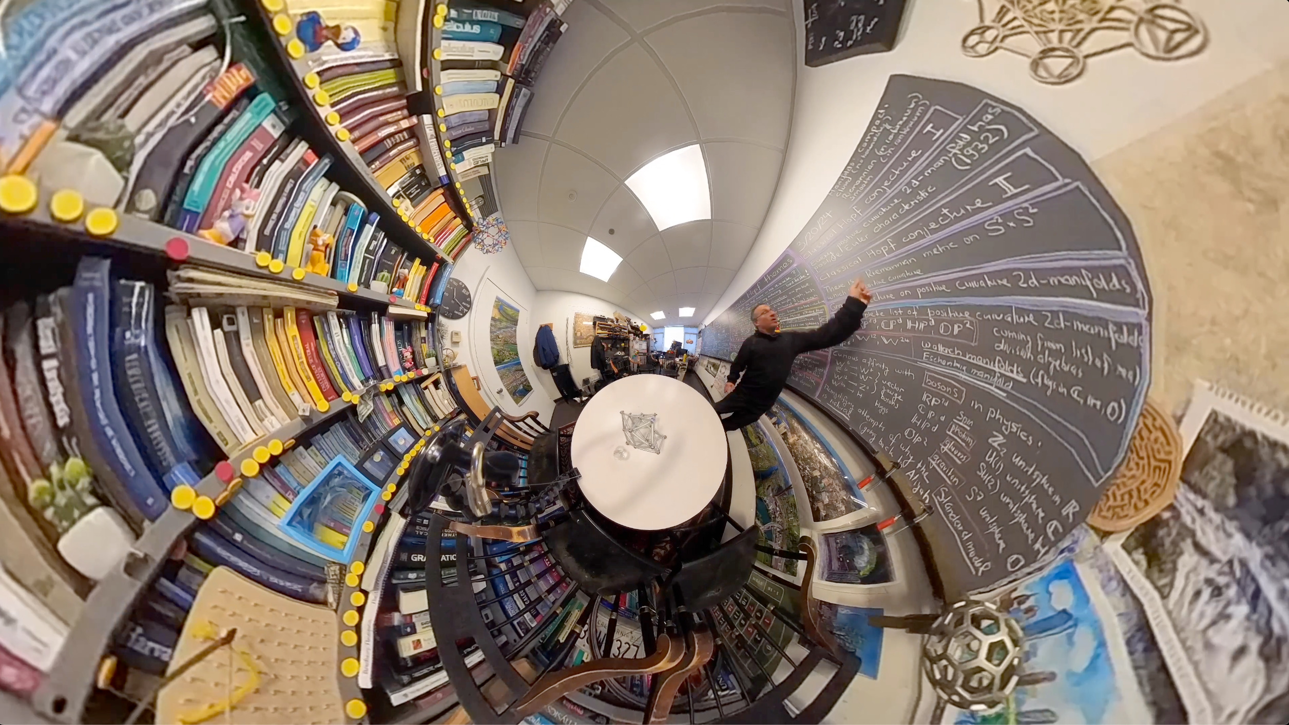
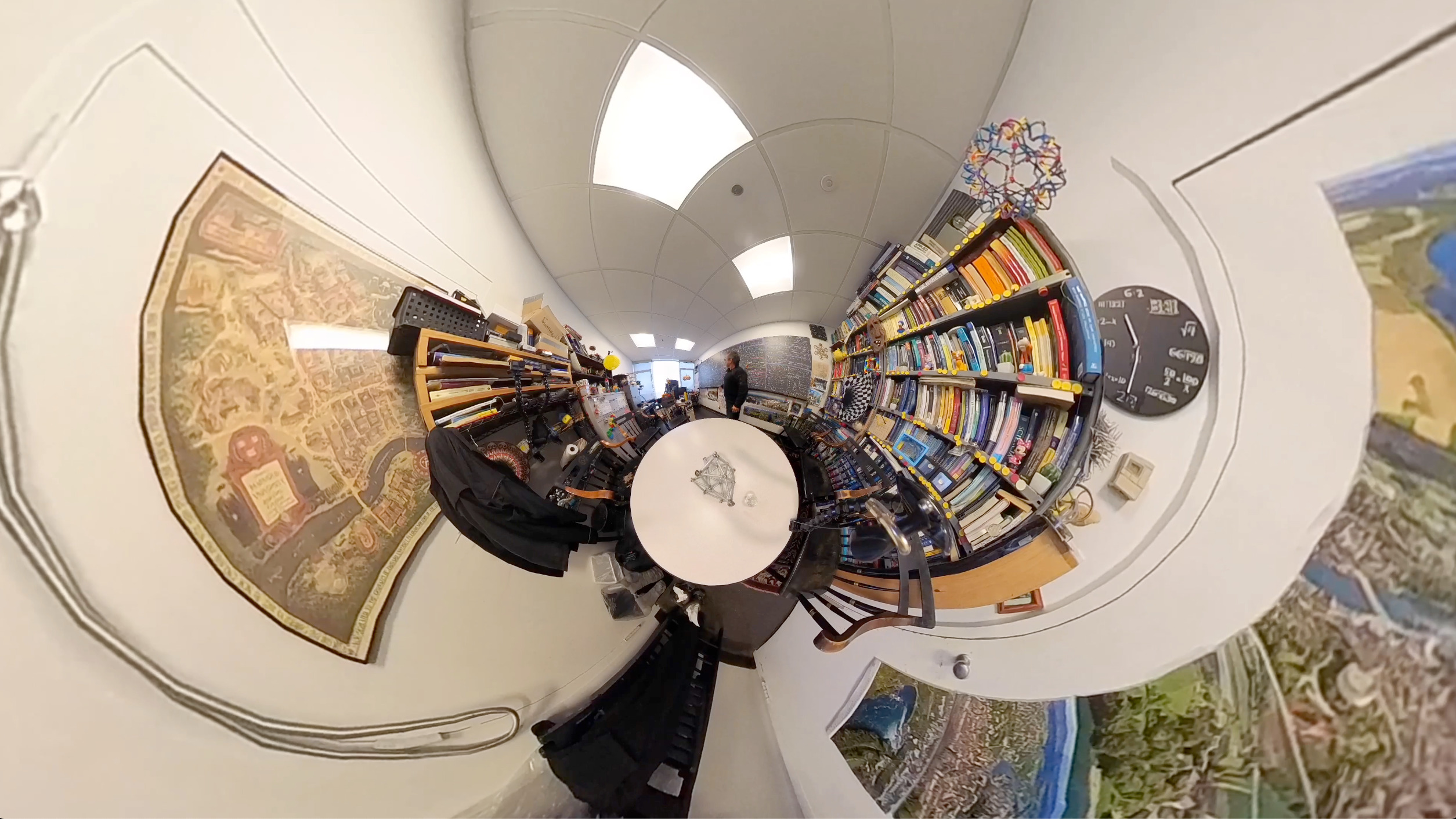
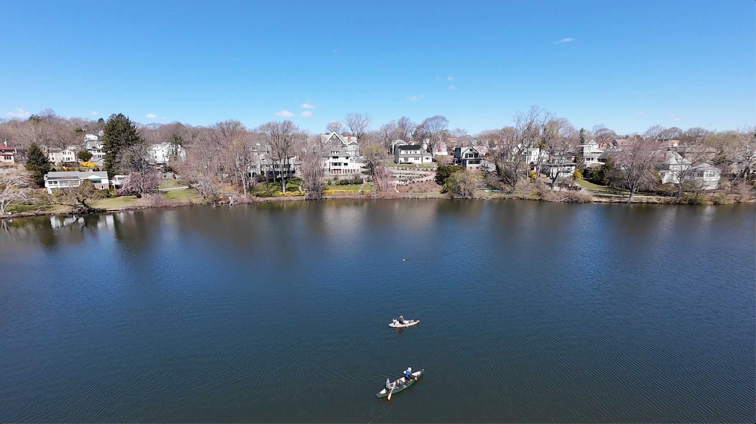
Here is the video from Saturday. I felt a bit dramatic with all the Magnolia and Cherry Blossom trees outside and whether changing rapidly, hence the organ music for this organic day (Saturday however sucked with lots of rain). The pictures were shot with the new Avata 2.