Energy theorem for Grothendieck ring

Energy theorem

The energy theorem tells that given a finite abstract simplicial complex G, the connection Laplacian defined by L(x,y)=1 if x and y intersect and L(x,y)=0 else has an inverse g for which the total energy $\sum_{x,y} g(x,y)$ is equal to the Euler characteristic $\chi(G)=\sum_x \omega(x)$ with $\omega(x) = (-1)^{dim(x)}$ . The determinant of $g$ is the Fermi characteristic $\psi(G) = \prod_x \omega(x)$ . In the “spring 2017 linear algebra Mathematica project (.nb)” the following self contained mathematica code was included:

CliqueNumber[s_]:=Length[First[FindClique[s]]];
ListCliques[s_,k_]:=Module[{n,t,m,u,r,V,W,U,l={},L},L=Length;
  VL=VertexList;EL=EdgeList;V=VL[s];W=EL[s]; m=L[W]; n=L[V];
  r=Subsets[V,{k,k}];U=Table[{W[[j,1]],W[[j,2]]},{j,L[W]}];
  If[k==1,l=V,If[k==2,l=U,Do[t=Subgraph[s,r[[j]]];
  If[L[EL[t]]==k(k-1)/2,l=Append[l,VL[t]]],{j,L[r]}]]];l];
W[s_]:=Module[{F,a,u,v,d,V,LC,L=Length},V=VertexList[s];
  d=If[L[V]==0,-1,CliqueNumber[s]];LC=ListCliques;
  If[d==0,v={},a[x_]:=Table[{x[[k]]},{k,L[x]}];
  F[t_,l_]:=If[l==1,a[LC[t,1]],If[l==0,{},LC[t,l]]];
  u=Delete[Union[Table[F[s,l],{l,0,d}]],1]; v={};
  Do[Do[v=Append[v,u[[m,l]]],{l,L[u[[m]]]}],{m,L[u]}]];v];
ConnectionGraph[s_]:= Module[{c=W[s],n,A},n=Length[c];
   A=Table[1,{n},{n}];Do[If[DisjointQ[c[[k]],c[[l]]]||
   c[[k]]==c[[l]],A[[k,l]]=0],{k,n},{l,n}];AdjacencyGraph[A]];
dim[x_]:=Length[x]-1; Pro=Product; F[A_]:=A+IdentityMatrix[Length[A]];
Euler[s_]:=Module[{w=W[s],n},n=Length[w];Sum[(-1)^dim[w[[k]]],{k,n}]];
Fermi[s_]:=Module[{w=W[s],n},n=Length[w];Pro[(-1)^dim[w[[k]]],{k,n}]];
ConnectionLaplacian[s_]:=F[AdjacencyMatrix[ConnectionGraph[s]]];
Fredholm[s_]:=Det[ConnectionLaplacian[s]];
GreenF[s_]:=Inverse[ConnectionLaplacian[s]];
Energy[s_]:=Total[Flatten[GreenF[s]]];
s=RandomGraph[{23,70}]; Print[Fermi[s]==Fredholm[s]];
{Euler[s],Energy[s]}

[Mathematica serves well as Pseudo code if one avoids functorial language parts like \. & @. The procedure W which gives the Whitney complex is compressed by purpose. (For somebody who does not like compressed code, the compactifiction is easy to expand in a few seconds. On the other hand, meandering long “poem style code” or worse (library code) is difficult to compress.) The procedure collects the complete subgraphs and that is known to be a hard problem. I have also used the external IGraphM libraries in the past but try to avoid libraries as most depreciate and break code rather quickly (typically in a few years) Having been programming in mathematica since 30 years, I kept all my old code. Almost all programs which have used external libraries are broken now, almost everything which did not use external libraries still work or were easy to adapt as the language evolved from “mathematica 1” to “mathematica 11” (some of us students at ETH had versions of mathematica for testing reasons before it officially was sold). There had been a nice combinatorial package for example which is so incompatible now that I had to write mathematica code which wrote mathematica code, ran it sandboxed by the side with the library and then reloaded the result as the library broke essential other parts. (Most of the combinatorial package is now built into the language but not all!). In other parts of computer science the importance of independence has been realized too: the development of docker for example illustrates how to avoid dependencies hell by building independent containers. Dependency hells in early Linux distributions are an other example.

The energy theorem also made a cameo in a Exam (problem 7) of spring 2017. The complex there is the set of all subsets of a 2 point set. The complex has Euler characteristic 1 and Fredhholm characteristic -1 (as there is an odd number of odd dimensional cells). In that problem, both the Laplacian L and the Green function g were given as concrete 3 x 3 matrices. We gave the eigenvectors of L. The task was to find the eigenvectors and eigenvalues of g. There is almost nothing to compute there. Still that problem turned out to be the hardest in the exam (simple things are often hard to spot).

Extending to the Grothendieck ring

The energy theorem goes over to the Grothendieck ring of cellular complexes. The Grothendieck ring is defined similarly as in the continuum but it has nothing to do with the ring of networks mentioned earlier. That ring of networks featured an addition (the Zykov join operation) and multiplication (newly constructed) which left the category of simplicial complexes or the category of finite simple graphs invariant. The Grothendieck ring has the disjoint union as an addition and a product which is only a cell complex and not an abstract simplicial complex any more. The Euler characteristic extends to a group homomorphism from the ring to the integers. We will see that every element in the ring has a Laplacian L with inverse g such that the energy $\sum_{x,y} g(x,y)$ is the Euler characteristic.

[April 23 update: the fact that the energy is a ring homomorphism follows already algebraically from the following lemma:

Lemma. If G,H are two cellular complexes and G x H is the ring product, then the Fredholm connection Laplacian of G x H is the tensor product of the Fredholm connection Laplacians G and H. The same is true for the Green function matrices, the inverse matrices.

Corollary. Energy is multiplicative.

Since tensor product has the total sum of the matrix entries is multiplicative, energy is multiplicative. We can not directly claim from this that energy is Euler characteristic as it is not obvious that energy is a valuation satisfying $E(A \cup B) + E(A \cap B) = E(A) + E(B)$ .

An other important corollary is the following multiplicative property of the spectrum of the connection Laplacian.

Corollary. The eigenvalues of the connection Laplacians multiply. If $\mu$ is an eigenvalue of the connection Laplacian of G and $\lambda$ is an eigenvalue of the connection Laplacian of H, then $\lambda \mu$ is an eigenvalue of the connection Laplacian of the connection Laplacian of the product complex G x H.

End update]

The definition of the ring

I’m not aware that the Grothendieck ring has been considered in a combinatorial setup, where one refuses any Euclidean notions or infinity. [The combinatorial attitude is in the spirit of quantum calculus. The continuum analogue which comes closest is the Grothendieck ring of varieties. The abstract in this paper (B. Poonen, Math. Res. Letters 9 (2002), no. 4, 493â€“498) gives a concise definition for the later. The result in the Poonen paper suggests that also the multiplication in the discrete Grothendieck ring does not give a unique prime factorization but since that paper goes deep into pretty heavy mathematics this is far from clear.] The Grothendieck ring of complexes we are going to look at is related to an extension of the Stanley-Reisner ring. But not for all elements in the algebraic ring, the energy theorem holds. We really need a CW structure, as when building up the complex, we have to be sure that the boundary of a newly attached cell is is a discrete sphere (in particular an object with Euler characteristic 0 or 2). In order to verify the energy theorem, one then only has to show that the product of discrete CW complexes is again a CW complex but that can be done by induction. The Grothendieck ring can not be defined on the category of abstract simplicial complexes as the product of two complexes fails to be an abstract simplicial complex.

[About the history: Gerald A. Reisner was a student of Mel Hochster. Reisner wrote a thesis on Cohen-Macaulay quotients of polynomial rings in 1974 under the guidance of Hochster. The name Stanley-Reisner ring is established now, even so Hochster should probably also be included. Polynomial rings have been studied before (Francis Macaulay in 1916 or Irvin Cohen in 1946 but the Stanley-Reisner picture is the implementation of that structure on a combinatorial level for a simplicial complex). The thesis “Grothendieck Ring of Varieties” of Neeraja Sahasrabudhe tells a bit about the history of the ring of varieties. It seemed have appeared first in a letter of August 16, 1964 of Grothendieck to Serre.]

In order to define the product in the Grothendieck ring, one first has to extend the category of finite abstract simplicial complexes to something which is closed under the Cartesian product operation (without doing the Barycentric refinement steps as we did to get the graph) A discrete analogue of CW complexes will do. We have looked at this structure already in an earlier entry. The definition very much relies on a good notion of what a “sphere” is. The notion of Evako sphere works best, better than discrete Reeb sphere notions considered earlier in discrete Morse theory. We have in this paper looked at a Cartesian product of graphs which gives again a graph. With the product to be defined shortly, it is $(G x H)_1$ which is a graph. The product defined in the Kuenneth paper is not associative as $G \times (K_1 \times K_1)) = G_1, (G \times K_1) \times K_1 = G_2$ . [One could look at equivalence classes of graphs, where $G \sim H$ if one is obtained from the other by applying Barycentric refinements. Since we want to compute in the ring on the computer we can not accept such identifications.] The fact that the product of two finite abstract simplicial complexes is not an abstract simplicial complex any more is already evident in the simplest cases. Let $G=K_2 \times K_2 = \{ (A,B) \; | \; A \in K_2, B \in K_2 \}$ is not an abstract finite simplicial complex as $(A,\emptyset)$ is not an empty set but not included in the product.

The theorem

For every element G in the Grothendieck ring R of cellular complexes, the connection Laplacian L has an inverse g whose total energy sum is equal to the Euler characteristic of G. Energy is therefore a ring homomorphism from the ring R to the integers.

Writing this up essentially consists of doing the discrete CW construction then carry over the proof of all the results to this structure. There is no new idea needed as all proofs rely on CW construction ideas (add a cell and see how the Fredholm characteristic or the energy changes) and all this relies on discrete additive and multiplicative Poincaré-Hopf formulas. Furthermore, every element G in the Grothendieck ring still has a connection graph G’ as well as a Barycentric refinement graph G₁ attached to it. The fact that the Euler characteristic is multiplicative is even true on a cohomological level, as Kuenneth shows.

Example 1

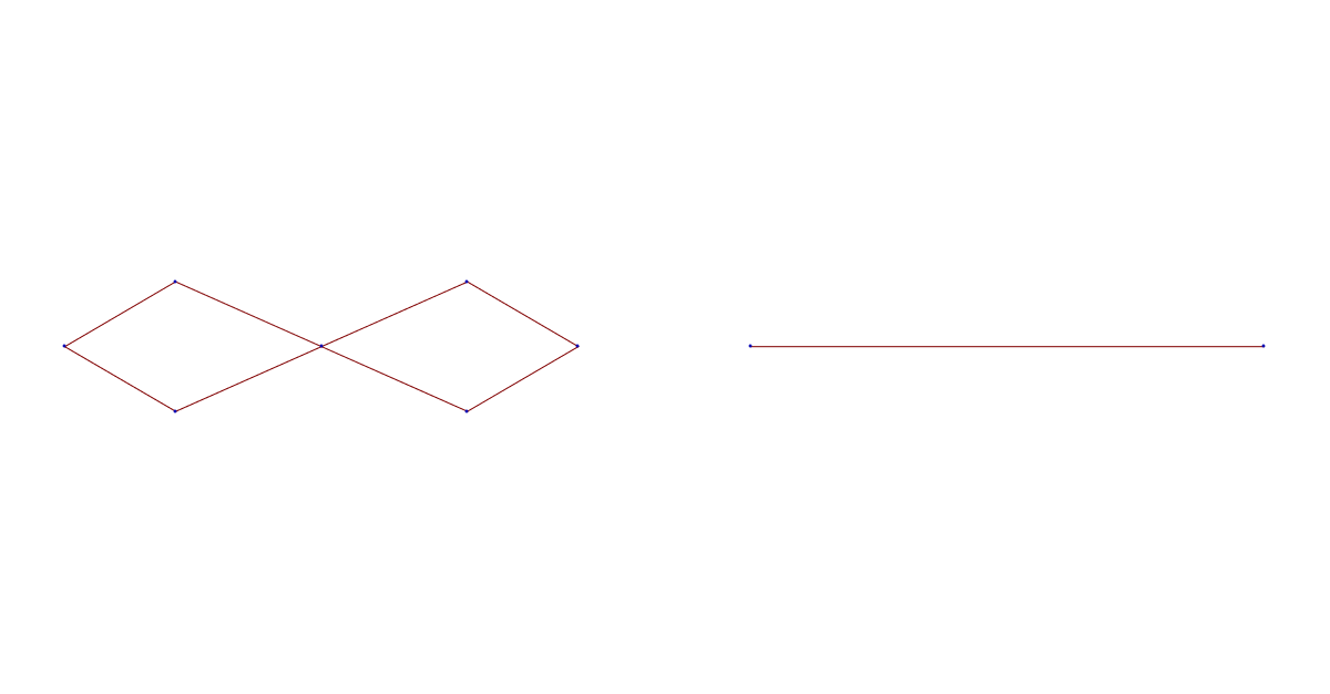
Let G₁ be the Whitney complex of the figure 8 graph. It has Euler characteristic -1. The graph G₂ is the complete graph K₂.

The connection graph G’ of the product G = G₁ x G₂ is shown here:

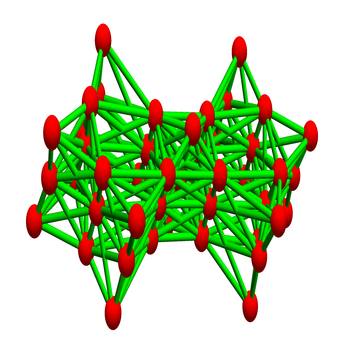
It has (7+8) (2+1)=45 vertices. The inverse of the connection Laplacian (the Green function) is here:

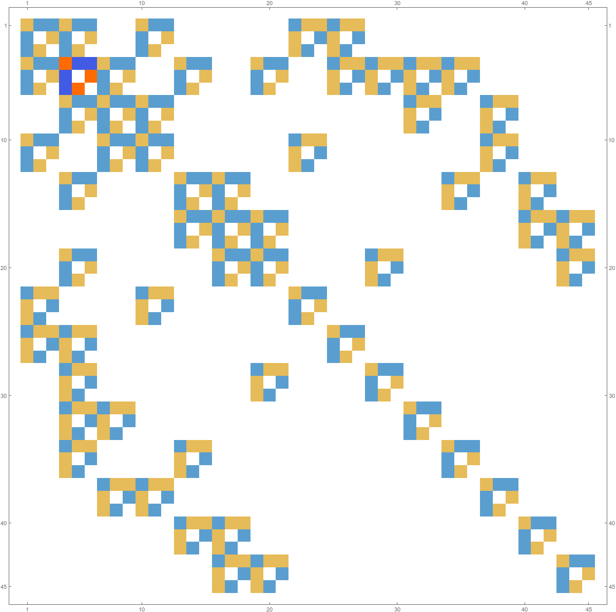
The total sum over all entries is indeed -1, which is the Euler characteristic of the product complex.

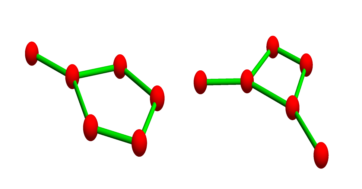
Example 2

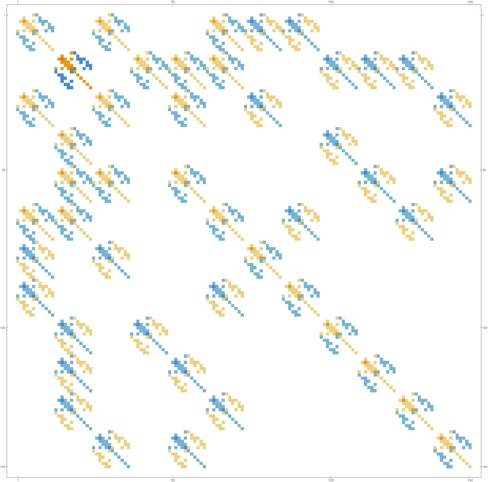
Here we have two one dimensional graphs, both with Euler characteristic 0. The graphs represent their Whitney complex. Both complexes have maximal dimension 1 and have 12 cells each.

Here is the connection graph of the product complex (a complex with 144= 12² cells). The connection graph is one way to visualize the complex (a set of finite non-empty subsets closed under the operation of taking non-empty subsets). But we made the point above that this product complex is not realized as the Whitney complex of a graph. We had to go beyond abstract simplicial complexes to have this product. In the Kuenneth paper, the first Barycentric refinement was taken to be able to work with complexes. This is a graph but the prize to pay is the loss of associativity in the product. In that paper we had seen the product related to the Stanley Reisner ring multiplication (which is associative), but when working with the ring too, one does not make the Barycentric refinement step. The Stanley-Reisner ring is an algebraic analogue but it is too large. There are elements in the ring which correspond to a larger class of simplices, a class of simplices where the boundary of cells are not necessarily spheres.

And here is the Green function g(x,y) of the product. It is a 144 x 145 matrix: