
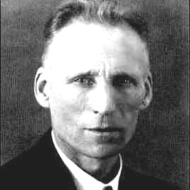
In algebraic topology one knows the structure of a CW complex. In that acronym, “C” stands for “closure finite” and “W” for weak. It could as well stand for “Constantine Whitehead” as the structure was developed by John Henry Constantine Whitehead in a sequence of papers published in 1949 and is used in every introductory course in algebraic topology. [I myself was exposed to CW complexes first in a course of Dan Burghelea, he gave at ETH in 1985. As that course had been read in French, CW complexes are for me therefore still “complex cellulaires”. By the way, my hand written notes of that course are here [18 Meg PDF]. ]
Even so, finite CW complexes have a finite combinatorial structure, the common theme is so see them as a construct in which a repeated “addition of handles” has taken place: start with a Hausdorff topological space X and attach cells = balls to it. First take an embedding f of a sphere Sn-1 into X, then build the quotient topology of the disjoint union of X and the ball Bn where points x in Sn-1 ⊂ Bn and f(x) ∈ X are identified. This process is called the attachment of a n-cell.
One can start with the situation, where X0 is a finite discrete set, then first attach a finite number of 1-cells. We end up with a one-dimensional complex X1, the 1-skeleton of the final construct. Now attach a number of 2-cells. We end up with a two dimensional complex X2. After finitely many such constructs, we end up with a d-dimensional cellular complex. Finally one define a CW complex as a topological space which is homeomorphic to such a construct. Most spaces we know in geometric analysis are of this type. Note that the definition just given is a bit more special than needed. One can define inductively a CW complex as a topological space Y which is obtained from an other CW complex by attaching a cell. The induction assumption is that a finite set with the discrete topology is a CW complex. Note that by this definition, the order with which cells are added can matter, as we can build additional cells on parts which have previously been added. The notion of CW complexes is not as general as the notion of a general Hausdorff topological space; but it generalizes the notion of a topological space equipped with a simplicial complex structure or in particular a manifold.
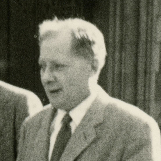
Even in this finite setup, standard (n-1)-spheres and n-balls in Euclidean space are used for the definition.It in particular assumes the “infinity axiom” in the ZF. I myself completely accept the ZFC frame work, but why use infinite constructs to describe objects which are finite and combinatorial? A mathematician who formulated the concerns skillfully is Luitzen Egbertus Jan Brouwer. While I don’t share his concerns too much on a fundamental level, it is still important to develop a finite mathematics independent of such consistency considerations ([I personally got aware of such issues through lectures of Erwin Engeler, a student of Paul Bernays, who not only taught a wonderful set theoretical topology course at ETH (Here are my notes [PDF]), but also other courses like theory of computation and mathematical software (My notes [PDF]). He once told me (in a casual hallway conversation) about “finitism” and “strict finitism” ideas, a theme about which he has published.]. There are also practical computer science reasons, when implementing the structures on a computer. More serious is the prospect of a worst case scenario: the emergence of a contradiction in the ZFC axiom system for example. By Goedel’s second incompleteness theorem, we can not prove the consistency within that system. Until now, we have not found a convincing and generally accepted larger frame work in which the consistency of ZFC can be proven. Anyway, also such a proof would hardly be reassuring as by the incompleteness theorem again we would face the problem to convince ourselves of the consistency of that larger framework within an even larger one. A simple way out of this frustrating “Its turtles all the way down” problem is to not even to start setting the foot into the mud and stay if possible within finite mathematics.
So, lets put ourselves into the shoes of Brouwer and work with finite structures. It allows us to enjoy the benefit that whatever we do, can be implemented in full detail on a finite computing device, as long as the structures are small enough. In order to define a CW complex in the discrete, we need a notion of a “sphere”. The simplest combinatorial structure where spheres appear are when looking at boundaries of simplices of finite abstract simplicial complexes.The later is a a finite set V on which one has given a finite set G of non-empty subsets such that if ∈ G, and B ⊂ A, then B ∈ G. The sets in G are the simplices. Again, since many texts treat simplicial complexes through their realization in Euclidean space we have to stress that a finite abstract simplicial complex is a finite object valid for somebody who thinks the concept of infinity should go to hell.
A convenient and intuitive way to generate finite simplicial complexes is to use a finite simple graph G=(V,E) as a background. Graphs are convenient as they are intuitive and easy to work and program with. A graph G contains many different simplicial complex structures in general. The largest one is the set of all complete subgraphs of the graph. This is the Whitney complex of the graph. There are smaller ones, like G=V ∪ E, which is the 1-skeleton complex on the graph. It can be useful to use several simplicial complex structures on a graph especially in proofs as it gives more flexibility to deform the graph. There are many stages for example to get from a graph to a pyramid extension of the graph. With this point of view, a finite simplicial complex on a graph G is already a CW structure on a graph. The individual cells are the k-simplices. The boundary of a k-simplex is a union of (k-1) simplices which can be seen as a discrete sphere. It is a crude version of a sphere.
There is a nice notion of what a “sphere” is in a graph. The definition is inductive and due to Evako. It is for example used in in a formulation of Jordan Brouwer to which we refer also for references. (We came to this concept independently but the basic setup is due to Evako in the graph theoretical setup. Evako also make the homotopy theory in graph theory crystal clear. Again, also homotopy traditionally assumes a geometric realizations, requiring Euclidean spaces and so the infinity axiom. The Evako homotopy does not need any Euclidean space and would have made Brouwer happy.) One first defines in a completely combinatorial way what contractibility is. then, one defines a k-sphere inductively as a graph for which every unit sphere is a (k-1)-sphere and such that removing a single vertex renders the graph contractible. The induction assumption is that the empty graph is a (-1)-sphere. This definition implicitly assumes the abstract finite Whitney simplicial complex structure on the graph, meaning the set of all vertex sets of complete subgraphs. It can certainly be done for any simplicial complex structure imposed on a graph and especially for the 1-skeleton complex which in the 20th century was the default simplicial complex structure imposed on a graph (most graph theory books take this rather narrow point of view). The boundary of a triangle (complete K3 subgraph) for example is not a 1-sphere as the triangle and every subgraph of the triangle are contractible. There is a simple way to get an Evako sphere from a simplex. Just look at its Barycentric refinement of the simplex which is now a graph with interior and boundary. The boundary of the Barycentric refinement of a triangle for example is the circular graph C6. From the platonic solids (when considered as graphs), only the octahedron and icosahedron are Evako spheres. The cube and dodecahedron are one dimensional as for them, all unit spheres are zero- dimensional. The tetrahedron finally is three dimensional because all its unit spheres are two-dimensional.
A more general CW structure on a finite simple graph can be obtained again by “attaching cells”. First chose an Evako k-sphere in G, then build a pyramid extension (cone) over it. This produces a larger graph. But now, the newly attached vertex does not play the role of a vertex but of a k-simplex. While the new graph G’ is still a graph, we count the simplices differently. The connections to the new graph for example don’t count.
Definition: Given a finite simple graph G equipped with a simplicial complex C so that one can give an inductive notion of Evako sphere. A k-dimensional CW structure is a finite set of disjoint disjoint (k-1)-spheres. The union of the k-simplices as well as these spheres are the new simplices. Disjoint means that the spheres do not have a common simplex. More generally, a CW structure on a graph is a union of disjoint Evako spheres in G. The union of these spheres as well as set of all complete subgraphs forms now the simplex structure. It is not a simplicial complex any more but turns out to be good enough for geometry. The connection graph of a CW complex has the set of simplices of G as vertices. Two such vertices are connected if they intersect.
This structure appears naturally in a more general version of the unimodularity theorem. We have described the theorem a bit already in a Math table talk. Like any “nice” theorem, it equates two numbers, where the two sides are defined by two seemingly unrelated things: the first is algebraic: it is the Fredholm determinant
det(1+A(G'))
where A(G’) is the adjacency matrix of the connection graph G’ of G. It is a special value of a Bowen-Lanford Zeta function
ζ(z)=1/det(1-zA) associated to the geometric structure (here the adjacency matrix of the connection graph) and therefore a spectrally defined notion. The second quantity is the Fredholm characteristic which is defined as
φ(G) = ∏x ω(x)
which is a multiplicative version of the Euler characteristic:
χ(G) = ∑x ω(x) ,
where ω(x)= (-1)dim(x) is the parity of a simplex. The Fredholm characteristic is of more combinatorial nature. A physisist liking super symmetry would see the Fredholm characteristic as the determinant of the parity operator P on linear space of discrete differential forms. This operator appears for example in the notion of super trace as str(A) = tr(P A) for any operator on differential forms. In analogy one can define the super determinant by sdet(A) = exp( str( log(A) ) ) = det(P A). So
The Euler characteristic is the super trace of the identity: str(1) = tr(P).
The Fredholm characteristic is the super determinant of the identity sdet(1) = det(P).
The fact that the Fredholm characteristic is a Fredholm determinant det(1+A) for the adjacency matrix of the simplicial complex is concrete and explicit. Here is the theorem. It is now a bit more general than for simplicial complexes:
| Unimodularity Theorem: For a graph G equipped with a CW complex structure, the Fredholm determinant of the connection graph is the same than the Fredholm characteristic of G. It especially is an integer in {-1,1}. The adjacency matrix of the connection graph of a CW complex is therefore always unimodular. This implies that the inverse, the Green functions (1+A)-1ij of a complex is integer-valued and of topological interest. |
A special case is when G is a finite abstract simplicial complex. Even more special is if we have the Whitney complex of a finite simple graph. Now we discovered the theorem first experimentally in February 2016. It turned out not to be easy to prove. The Hammer and Chisle or Sledge hammer approach did not work well so far. We had to build up more theory and so use the “rising sea” approach. One of the necessary steps had been to extend it to more general structures than graphs. It might appear crazy first to to generalize something before settling the simpler case. The reason for generalization is that simplicial complexes or even CW complexes that they allow for a finer induction process. Adding a single vertex to a graph turns out to be a huge modification to a graph since many fnew simplices are added simultaneously to the graph. The corresponding linear algebra is difficult as we add many new rows and columns. Managing the determinant analogue to the Laplace expansion is difficult. Adding a single simplex one by one is much more convenient. Why then generalize it even more? There is an other reason than “fine graining the deformation tools”: more general structures also lead to more interesting Fredholm numbers instead of only -1 and 1. And when doing experiments, it can be hard to see structure when only 1 or -1 appear. The CW structure is not the most general one. The collection of Evako spheres can more generally be a collection of geometric subgraphs, graphs for which every unit sphere is an Evako sphere. A graph G with a collection of disjoin geometric subgraphs a generalized cell complex. Lets again give the definition and refrain from stating it for general simplicial complexes but just look at finite simple graphs equipped with the Whitney complex:
Definition. A generalized cell complex is a finite simple graph G=(V,E) with a collection W of simplex disjoint geometric graphs in G. A geometric graph in G is a subgraph for which every unit sphere is an Evako sphere.
The unimodularity theorem does not generalize to this general structure as the Fredholm functional φ(G) now can take values different from -1 or 1. In order to prove the unimodularity theorem we proved a lemma which tells what happens with the Fredholm determinant φ(G) if we add a new simplex. This lemma is crucial and very general. It does not require the attached cells to be spheres. It can be anything:
Fredholm determinant lemma: Let F be any generalized cell complex and G a larger complex in which either a new vertex or a new cell x has been added. Then
φ(G) = i(x) φ(F) where i(x) is the Poincare-Hopf index i(x) = 1-χ(S(x)). |
The lemma also immediately shows why the number f(G) of odd-dimensional simplices in G matters in the case of Whitney complexes or CW complexes. For odd dimensional “cells” x which have even dimensional spheres, we have χ(S)=2 so that then 1-χ(S(x) ) = -1. On the other hand, for even dimensional cells which have odd dimensional spheres, we have χ(S)=0 so that then 1-χ(S(x)) = 1. We see that the Poincaré-Hopf index i(x) is the key. It explains why the unimodularity theorem is true and why only the odd dimensional simplices count: they have even dimensional spheres.
[The following illustration was Added November 29:]
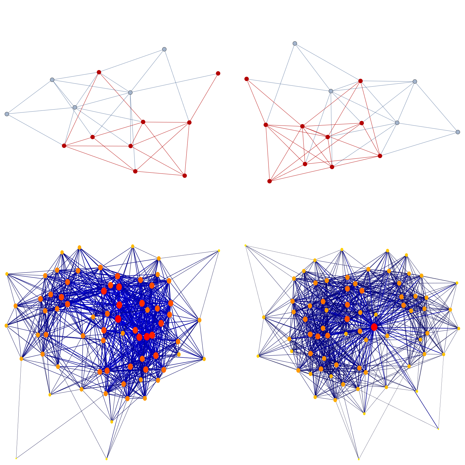
We see a random graph G with 14 vertices and Euler characteristic χ(G)=-4; Inside is a random subgraph with 9 vertices of Euler characteristic χ(H)=-2. The f-vector of G is (14,36,20,2) and χ(G)=14-36+20-2=-4. The f-vector of H is (9, 16, 6, 1) and χ(H)=9-16+6-1=-2; We see that H is far out from being a sphere (as spheres always have Euler characteristic 0 or 2). The first picture shows H highlighted as a subgraph of G. The second picture shows the pyramid extension Gx in which an additional vertex has been added. The f-vector of Gx is (15, 45, 36, 8, 1) leading to χ(Gx)=15-45+36-8+1=-1. The Poincaré-Hopf index of the new index is 1-χ(H) = 3. The Euler characteristic of Gx is confirmed by Poincaré-Hopf equal to -1. This is all nice and dandy. What happens with the multiplicative Euler characteristic? We needed a lot of experimentation to figure this out: the Fredholm extension lemma tells that the Euler characteristic of H (not the connection graph of H, which might have a different Euler characteristic in rare cases [this is related to the fact that connection graphs are in general not homotopic to the graph but in many cases actually are like after a Barycentric refinement]) matters. in that particular example here for example, the Euler characteristic of H is -2 as it is also the Euler characteristic of H’ which is a much larger graph with 32 vertices, 190 edges. Also comparing the Fredholm determinant of G’ and Gx‘ is not the right thing! Again, devilishly, it produces the correct identity in most cases and I myself believed for a while that it would work as such. Only failing to prove it forced me to reexamine the experiments and refine the picture.
We really have to think like Whitehead in order to see it! The Fredholm extension lemma can only be understood using CW complexes.
The picture is that the added vertex x over H is the process of having attached a new cell to the CW complex. On the level of graphs (Whitney simplicial complex of course), the extension lemma would be wrong as the join over H (pyramide or cone extension) would add a lot of more simplices which add a lot more paths to the path integral picture and distort the Fredholm determinant. What also helped is to work with more general cells and not only spheres for which the Euler characteristic i(x)=1-χ(H) has absolute value 1. Having more variety in the numbers make experiments sharper and allow more quickly to weed out wrong paths. In the case of the picture seen, the Fredholm connection determinant, the Fredholm determinant of G’ is equal to 1. The Fredholm determinant of the expanded cell complex G” has Fredholm determinant 3. The following picture shows the two matrices for the graph G’ (the CW complex obtained from the Whitney simplicial complex) and the CW complex G” of the extension for which we have just computed the Fredholm determinant. The fundamental Poincaré-Hopf-Fredholm Lemma implies that 3=φ(G”) = i(x) φ(G) = 3*1. This is the case here. Of course one only gets impressed by this if one tries it out with arbitrary graphs G and subgraphs H, thousands or millions of them until one gets confidence to actually prove it.

[End of addition]
For the Euler characteristic, there is the Poincaré-Hopf theorem. It defines the Poincaré-Hopf index of a vertex of a graph as i(x) = 1-χ(S(x)) where S(x) is the unit sphere. If we have a generalized cell complex given by a finite simple graph G=(V,E) together with a collection W of geometric disjoint subgraphs of G, define for x in V, the Poincare-Hopf index as before and for x in V, representing a subgraph S(x) of G, define i(x) = 1-χ(S(x)), the Poincaré-Hopf index of the cell x. The Poincaré-Hopf theorem tells χ(G) = i(x) + χ(F) in the graph case. How to define Euler characteristic in the case of generalized cell complexes? It is quite easy to see that if we want the Euler characteristic to remain a valuation satisfying χ(F ∪ G) = χ(F) + χ(G) – χ(F ∩ G), then we better have to define it through the Poincaré-Hopf theorem.
Definition. The Euler characteristic χ(G) of a generalized cell complex G is defined as ∑ x ∈ V ∪ W i(x), where i(x) = 1-χ(S(x)), where for a vertex x ∈ V, S(x) is the unit sphere in G and where if x ∈ W, S(x) is the geometric graph under consideration.
Now, we have an other indication why the Fredholm characteristic is a cousin of the Euler characteristic: For any generalized cell complex, we have
  χ(G) = ∑x i(x)         (Poincare-Hopf)
  φ(G) = ∏x i(x)        (Fredholm Lemma)
In particular, for a CW complex or abstract finite simplicial complex, where i(x) = 1-S(x) ∈ {-1,1}, φ(G); ∈ {-1,1}, the adjacency matrix of the generalized cell structure is unimodular. In other words, the multiplicative Poincaré-Hopf result makes things more transparent. In general, for a generalized cell complex, as the Fredholm determinant φ(G) is then no more necessarily -1 or 1. It would be nice to know how large the set of graphs is which can be seen as a connection graph of some generalized cell complex of this type. We actually believe it to be possible that there is an even larger generalization of generalized cell complex (completely parallel to surgery constructions in the continuum) in which the order of the attached cells matters so that we can reach any graph as a connection graph and have the Fredholm lemma (a multiplicative Poincaré-Hopf theorem). But this requires to understand a more complex Morse story. I’m optimistic because the multiplicative Poincaré-Hopf result works very well in full generality, where the attached cell is even over an arbitrary subgraph (and not just a sphere like for CW complexes or geometric graphs like for generalized cell complexes). What has still to be checked that with the definition of Euler characteristic given the indices of newly attached handles work. In classical Morse theory, we start with the geometric object (like graph or manifold), then chose an order of the points (using Morse function), then build up the CW structure. Now for graphs, the Morse theoretical build-up does not have to attach disks, one can attach pretty much everything and the Morse indices can be pretty arbitrary (unlike for Morse functions, where the Poincaré-Hopf indices are -1 or 1). This is what surgery constructions in the continuum are about. For the generalized cell structures build up, chosing a different order of the build-up produces a different structure. In some sense, it is a non-commutative Morse theory. The Poincaré-Hopf theorem still holds but it is not a theorem about a function on the geometric graph but about an ordered sequence of attached cells. The notion “generalized cell complex” given here is special still in the sense that the order in which the attached cells are added does not matter. The Poincaré-Hopf theorem as well as its multiplicative cousin, the Fredholm Lemma are both a theorem in that case. What we don’t yet know for sure (because we have not implemented it in the computer) is whether the theorem holds for a very general non-commutative Morse set-up, where the order of the addition of the general cells matters, allowing to be built on already built generalized cell structure.
An other parallel result between Euler characteristic and Fredholm characteristic are the valuation relations:
 χ(F ∪ G) + χ(F ∩ G) = χ(F) + χ(G)  (additive valuation)
 φ(F ∪ G) φ(F ∩ G)   = φ(F) φ(G)    (multiplicative valuation)
A generalized cell complex has also a natural cohomology.The new ideal spheres S(x) do not have to be closed oriented geometric graphs. We can still define the exterior derivative df(x) = f(S(x)) satisfying d2 = 0.
Once one has a notion of index, one can define curvature as the expectation of the index with respect to some averaging measure. We have explored this for a while now
- Index expectation (2012)
- Index formula for graphs (2012)
- Coloring graphs using topology 2014
- Gauss Bonnet for valuations 2016
There are various ways to generate probability measures of indices. On graphs, where indices are defined by locally injective functions, we can just look at probability spaces of functions for which almost all functions are locally injective. An other source for random geometric structures are determinants. If we look at the Fredholm determinant of a graph, then this is in some sense a partition function over all one dimensional CW complexes which can exist on a graph. The kicker was that since the Fredholm determinant is a sum over the Fredholm characteristics over all these oriented one-dimensional CW complexes on the connection graph. The unimodularity theorem assures that this is the Fredholm characteristic of the graph.
How do we define then curvature for Fredholm characteristic naturally? We don’t know yet. First we need to finish writing up the paper. In any case, we think the definition of curvature in a very general setup is not much harder. In the case of a graph or finite abstract simplicial complex or generalized cell complex as defined here, it is pretty clear as we just have to average over all possible built-ups of the space. In the case of graphs, we for example just can average over all possible locally injective functions. To define curvature for an even more general cell complex, we have average the indices when summing over all possible build-ups of the structure. In any case, whenever there is a Poincare-Hopf theorem, there is also a Gauss-Bonnet theorem telling that the integral over all the curvatures is the Euler characteristic. The multiplicative version is that the product of the Fredholm curvatures is the Fredholm characteristic.
We currently hope that any finite simple graph can be the connection graph of a generalized cell complex. The Fredholm determinant of the graph itself has Poincare-Hopf and Gauss-Bonnet formulas. Compare that in the unimodularity theorem, where we currently only look at the Fredholm determinants of connection graphs of CW complexes. For a general graph, the Fredholm determinant seizes to be {-1,1} valued and can be pretty arbitrary. If this works, then it would be worthwhile to consider a generalization of the textbook definition of CW complex in which in each case, not a cell (k-ball) is added but a rather general cone of an arbitrary CW complex can be added. The classical CW complex is the special case where the boundaries of the cells are spheres. In any case, such a more general structure remains reasonable as there is a Gauss-Bonnet theorem for it as well as a natural cohomology as well as Laplacians, Hodge theory etc. This looks like a huge program but in reality it all exists already as we have these structures for general finite simple graphs. Its just that our point of view has shifted and graphs are more emancipated: while in the 20th century graphs were mostly treated as one-dimensional simplicial complexes, topologists like Whitney, Fiske, Evako, Forman looked at graphs as more general topological constructs featuring richer simplicial complex structures. Now, graphs have general Poincaré-Hopf, Gauss-Bonnet, Brouwer-Lefschetz theorems. What we start to see now is that we can look at general graphs as connection graphs of a rather large class of topological spaces obtained by adding rather general handles. But the litmus test is not beauty or generality, but whether theorems work. In our case, the question is whether we can write in general the Fredholm determinant of a graph as a product of Poincare-Hopf indices. Now, in a naive way this is certainly wrong as for most Morse functions, there are many regular points for which the Poincare-Hopf index is zero. The product of the Poincaré-Hopf indices is therefore zero in most cases. But the Fredholm determinants are mostly nonzero. The naive point of view can not be more wrong.
What emerged again through the analysis of the unimodularity theorem is that we have to look at a graph not as something per se but as a shell on which more structures can be built. This is well known in mathematics. The set of real numbers as a set are pretty boring. It is just an uncountable set without any interesting structure (order structure, topology of open sets, δ-algebra of measurable sets) yet. For a graph, we can first of all pop-up a simplicial complex structure. There are many. There is the one dimensional skeleton given by the union of vertices and edges, then there are others up to the Whitney complex. But there are more structures possible besides simplicial complexes. CW complexes lead the way. For example, we can see the Wheel graph W4 (with 4 spikes) as a connection graph of a 2-cell even so the connection graph of any graph which is a 2 cell is much bigger. The connection graph of a triangle for example (the smallest two dimensional cell) has already 7 vertices.
Now, and this can be shocking at first, the additional geometric structure also can change the Euler characteristic of the structure. For example, if we look at the tetrahedron graph K4, then with the Whitney complex C, the Euler characteristic is 1 as there are 4 vertices, 6 edges and 4 triangles and one 3-simplex. So that χ(G,C)=4-6+4-1=1. If we look at the the graph K4 however equipped with the 2-skeleton complex C, then the 3-cell does not count. The Euler characteristic is now χ(G,C)=2 (as Descartes and Euler would have counted the Euler characteristic using the famous formula v-f+e=2, the Euler gem). Now, a graph theorist of the 20th century looks at the tetrahedron even as a completely different beast, namely a one dimensional simplicial complex C (essentially all textbooks take this point of view). Now the triangles do not count and the Euler characteristic is χ(G,C)= e-f = 4-6 = -2. The picture is now that one sees a sphere with 4 holes punched into it). This is an additional confusion which could well be mended into the Lakatos discussion about one of the most embarrassing stories in the history of mathematics, the fact that Euler gem theorem was not only once but several times “disproven” with counter examples. The first counter examples were of course the Kepler solid which fail to have Euler characteristic 2 in general. Today we know that the notion of “polyhedron” was muddy over the course of centuries. [There are many analogue confusions in mathematics and they are all based on ambiguities. For example: as paradoxa like Bertrand’s paradox in probability theory indicate, that the notion of probability is not just an intrinsic notion of a space, but depends on additional structure: not only the σ-algebra but also from the probability measure. Notions like entropy can confuse as it is a matter of fact that all basis laws of physics we know are reversible so that entropy stays constant but then there are laws of thermodynamics claiming that the entropy increases. This is not a paradox if one understands to look at it with more structure, with structures for example which have emerged in the last century like martingale theory. ]
Any way, what we see now that there are lots of more cellular structures possible on a graph. Simplicial complex structures or CW complex structures make up only a small part. There appears first a slight difficulty in defining the Euler characteristic of such a structure as we can not just count cells any more. Note that the cells are now pretty arbitrary graphs with pretty arbitrary topological features and not necessarily bound contractible cells like in the case of simplicial complexes or CW complexes. Our suggestion is to use Poincaré-Hopf inductively to define the Euler characteristic. This has first of all the advantage that the Euler-Poincaré theorem is trivial as it is the definition. Only in the case of simplicial complexes or in particular the Whitney complex on a graph it becomes a theorem as it claims there that the result is independent in which order the structure has been built up. So, what is new now with the more general structures is that the Euler characteristic not only depends on the space but also on the Morse function as the later determines in which order the cells were added. What we don’t yet know is whether the multiplicative part of Poincaré-Hopf gives something which is independent of the structure and only depends on the graph. A more general unimodularity theorem would assure this. For now, the unimodularity theorem only holds for discrete CW complexes. For general cellular complexes, it gives an identity of the Fredholm determinant of the connection graph and the product of the Poincaré-Hopf indices. But that only applies so far if the additional cells are all disjoint so that the order in which the cells are added does not matter.
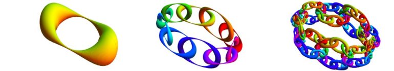
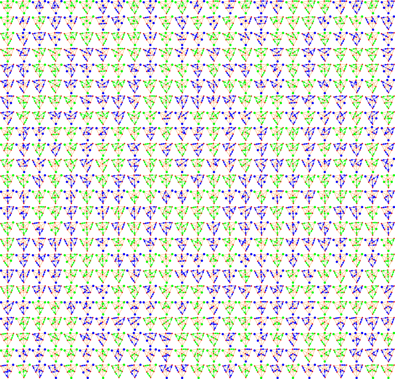
The following picture illustrates the unimodularity theorem. We look at a triangle for which the Fredholm characteristic is -1 (there are three odd dimensional simplices in the triangle, the three edges). The Fredholm determinant is already a path integral of a large number of closed paths. It is the set of all one-dimensional oriented paths in the connection graph G’ (which is larger than the Barycentric refinement). There are 601 such paths. 301 have odd signature and 300 have even signature. We see in the picture all except the empty path belonging to the identity permutation. It is absolutely non-trivial why the difference of these two classes is always 1 or -1. (By the way, in the Mathtable handout of this fall, we have mentioned that there are 90 paths which are transitive permutations of the vertices of the connection graph of the triangle G=K3. Fredholm determinants generate much more permutations as they don’t need to be transitive.)
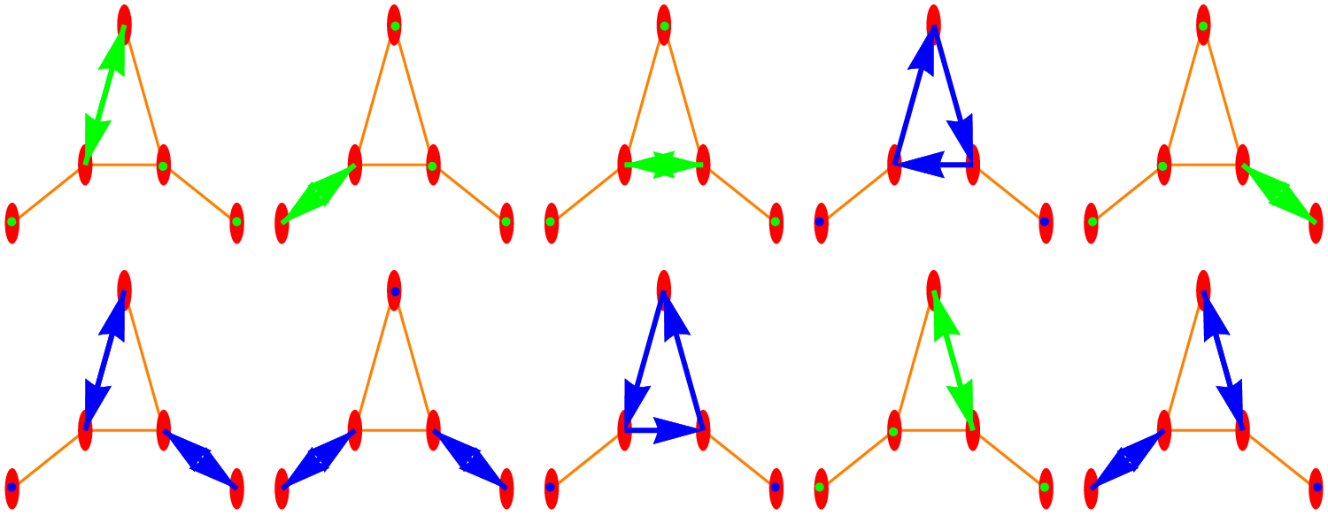
And here are all except the identity permutations belonging go the Fredholm determinant of the linear graph G of length 2. The connection graph G’ of G has 5 vertices, the 3 original vertices as well as the 2 edges. The two edges are connected to the central vertex producing a triangular K3 graph as a subgraph of the connection graph. We see that there 5 permutations which have odd signature and 6 permutations which have even signature. Indeed, the Fredholm characteristic is 1. as there are 2 odd-dimensional simplices in the graph. By the way, the unimodularity theorem is pretty easy to prove for one dimensional graphs G, graphs which have no triangles. The graph L3 treated in this example is one dimensional. Its connection graph is the bunny graph. The bunny graph was already featured in the math table handout about Wu characteristic.
By the way, Wu characteristic is closely related to the topic just discussed. We actually came to Fredholm determinants through Wu characteristic and intersection calculus.
And an other P.S.: the prime graphs appearing in the counting and cohomology story are naturally discussed in the context of discrete CW complexes. Actually the above multiplicative Poincaré-Hopf lemma allows to compute the Fredholm determinant of these graphs very nicely. They are just related to the products of the first n Moebius functions, the reason being that the Möbius functions are minus the Poincaré-Hopf indices of these graphs. Its important there to look at the CW complexes as the connection graphs of the prime graphs are much larger! CW complexes are just a perfect setting for understanding the Fredholm determinants of these graphs.
Added November 30, 2016: Here is a picture of the prime graph P(30) as introduced in the counting and cohomology paper. The vertices are the square free integers from 2 to 30. We have shown in that paper that counting is a Morse theoretical process:
|
Counting and cohomology theorem: The counting function f(n)=n is a Morse function the Barycentric refinement of the complete graph on the spectrum of the the ring Z of integers. The graph P(n)=(V(n),E(n)) has the vertex set V(n)={1 |
A naive thought is to try to estimate the growth of the Mertens function and so proving the Riemann hypothesis by estimating the Betti numbers, maybe through relation with curvature. As indicated in the paper, this certainly is not a silver bullet: first of all one has to establish curvature-Betti relations a la Gromov in the discrete, then estimate curvatures. A long fight could wait to clear that if at all possible.
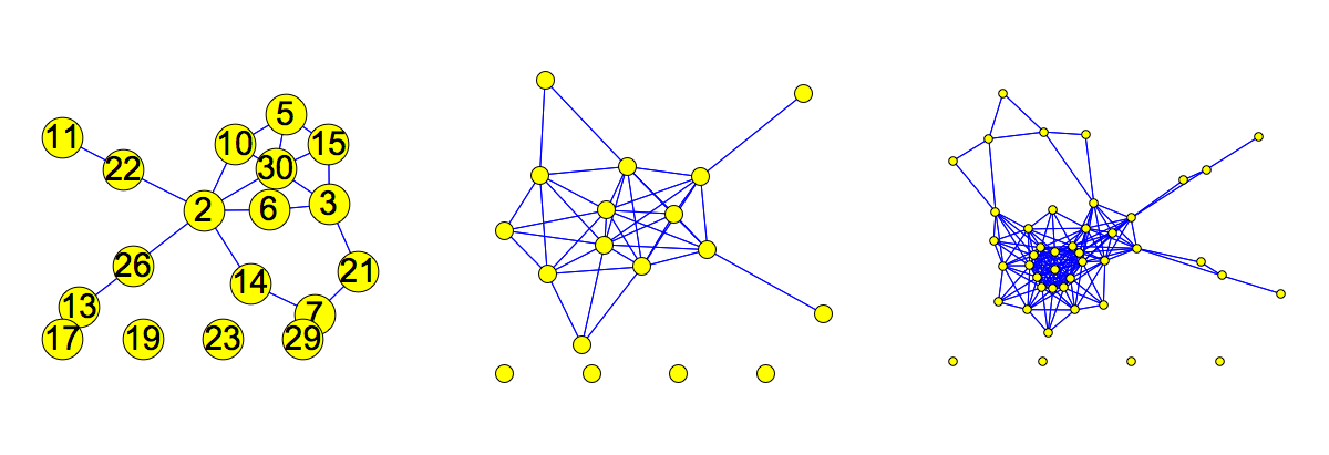
What is the multiplicative Euler characteristic = Fredholm picture? On one side one has the product of the Poincaré-Hopf indices, the Moebius function values. Now, according to the unimodularity theorem, this should be the Fredholm determinant of a connection graph. However, as just expressed in the above crucial lemma, this only works if we look at the graph P(n) as a CW complex; the reason is that adding a new vertex has to produce a new cell. In the next picture we first see the graph P(30), then an other graph and finally the connection graph P(30)’ of P(30). The third graph shown is larger as it contains as vertices all the complete subgraph of P(30). Yes, according to the unimodularity theorem, its Fredholm determinant is related to the number of odd dimensional simplices in P(30). As the f-vector of P(30) is (18,20,6) with Euler characteristic 18-20+6=4 which matches 1-M(30) = 1-(-3)=4, where M(n) is the Mertens function, the sum of the first 30 Moebius values {1, -1, -1, 0, -1, 1, -1, 0, 0, 1, -1, 0, -1, 1, 1, 0, -1, 0, -1, 0, 1,1, -1, 0, 0, 1, 0, 0, -1, -1}. The 18 nonzero values in that list (the first value 1 does not count because we don’t include 1 as a vertex as we would just get the unit ball of 1 which has always Euler characteristic 1 and is not interesting), are minus the Poincaré-Hopf indices.
Now lets look at the product of these Poincaré-Hopf indices. It is 1. This matches the Fredholm determinant of the connection graph. But thats pure luck (a 50 percent chance)! Indeed, when looking at the f-vectors of the prime graphs P(n), we see that the number of odd dimensional simplices are there always even. The Fredholm determinant of the connection graphs P(n)’ of P(n) are always 1. This is related to the fact that the prime graphs P(n) are “submerged parts” of a Barycentric refinement of a complete graph on the primes. Anyway, there is no Poincaré-Hopf match. But again, this is just because we did not think like Whitehead. The correct graph to consider is the CW complex. Now, every vertex of the prime graph is actually thought of as an attached cell. The vertex set is the same. But since we look at the connection graph (!), we have now to consider not at connections, where one integer divides an other but where two integers (x,y) have a non-trivial common prime factor meaning gcd(x,y)>1. This graph the second graph seen in the picture below. We call it the prime connection graph. These prime connection graphs are beautiful graphs too. But now, the Fredholm determinant of the adjacency matrix of this graph matches the product of the Poincaré-Hopf indices. This is the unimodularity theorem again, but now used in the more general context of CW complexes.
CW complexes have proven to be very useful also for practical reasons (i.e. cellular cohomology is much easier to compute in general than simplicial cohomology). It also leads naturally to a discrete Morse cohomology as mentioned in the counting and chomology paper too. But we have only scratched the surface by showing that for every graph, there exists at least one Morse function for which the Morse cohomology agrees with simplicial cohomology. There is no doubt that this holds in much more generality for the simple reason that the theory works in the continuum and because of the following quantum calculus principle: Everything which works in the continuum, works also in finite mathematics, sometimes even better.
End update of November 30.