

Can one hear the shape of a simplicial complex?
Update: November 27: One can hear the shape of a simplicial complex, ArXiv.
The connection Laplacian of a finite abstract simplicial complex G is the matrix L(x,y) = 1, if x and y intersect and 0 else. It is an unimodular matrix L whose entries of the inverse add up to the Euler characteristic. This is the energy theorem. It is this theorem which makes the connection Laplacian unique in its kind. If we look at adjacency matrices or Kirchhoff or Hodge Laplacians of discrete geometric spaces, we get kernels. The connection Laplacian has determinant 1 or -1 meaning that it is unimodular. The energy theorem tells us something: the Euler characteristic is a natural energy. We will see soon (even so not proven at the moment) that the energy can also be expressed as follows: assign a positive energy quantum to each positive eigenvalue and a negative energy quantum to a negative eigenvalue. The sum over all energies is again the Euler characteristic, the number of even dimensional minus the number of odd dimensional simplices in the complex.
The numerical computation of the energy of a complex is so short that it is tweetable. Since the connection Laplacian is so natural, there is hardly any way to wiggle the matrix without losing the unimodularity property, one is almost forced to ask:
| What geometric properties of a finite abstract simplicial complex can one hear from the eigenvalues of the connection Laplacian L? |
And this triggers the question
| Are there isospectral abstract simplicial complexes for the connection Laplacian? |
This question has been asked in 1966 for the Laplacian of a bounded planar region. In the case of graphs it has become an industry too leading to many classes of isospectral graphs. Here in the case of the connection Laplacian it has not been asked yet, probably as nobody has worked with the connection Laplacian of a simplicial complex yet. After having made some experiments, there is now also a small exhibit, where you can listen to some simplicial complexes.
Cultural background: can one hear the shape of a drum?
| It is by far the most important open problem in spectral theory: the question of Marc Kac of 1966. It is a question type. Once, the question about the relation between a spectral property and the geometric property of a geometric object has been asked one can consider it for all objects which have a Laplacian attached to them. Gordon-Webb examples have found isospectral drums but they are neither convex, nor smooth. Indeed, the Kac problem is wide open for smooth drums and it is wide open for convex drums. But the Gordon Webb counter examples fit the Kac question well as in that article, polygonal regions are discussed there prominently. |
|
In the Monthly article of Kac, it is also remarked that one can hear the area of a drum. At the very end, Kac mentions that one can hear the smooth holes for a smooth drum and asks the question whether one can hear the Euler characteristic of a drum. For the Laplacian of a smooth 2-dimensional manifold one can hear its Euler characteristic. As far as we know, it is unknown in general. Milnor had constructed the first examples of isospectral manifolds and they were also isospectral for the Hodge Laplacian which includes Laplacians on higher order differential forms.
Now, if we look at the Hodge Laplacian, then one can read off the eigenvalues by knowing how many there are in each sector of differential forms or also using a super trace like $str(1) = str(exp(-tL)) = \chi(G)$. But the super trace does not refer to the blank eigenvalues, which do not have a signature attached to them, whether they belong to a bosonic or fermionic eigenvalue. The same is also true for finite abstract simplicial complexes. We know the sum of the Betti numbers as this is the nullity of the Hodge Laplacian, but we don’t know the alternating sum which is the Euler characteristic again.
To summarize, both for manifolds or for graphs respectively finite abstract simplicial complexes the Hodge Laplacian does not determine the Euler characteristic yet (at least I’m currently not aware of a result like that). By the way, in the case of a k-dimensional drum, it would be very surprising to hear that the eigenvalues of the scalar Laplacian alone could give the Euler characteristic because the scalar Laplacian does not tap into the higher dimensional parts of space. But it is reasonable to ask whether the eigenvalues of the Hodge Laplacian do determine the Euler characteristic.
One can hear the Euler characteristic
The point of this blog is to point out on going research telling that there is now very strong indication that for a general simplicial complex, the spectrum of the connection Laplacian determines the Euler characteristic. Indeed: [late Oct 22, this is proven]
| The Euler characteristic of G appears to be the number of positive eigenvalues of $L$ minus the number of negative eigenvalues of $L$. |
This has been tested now in so many cases that it would be big surprise if it would fail. I do not know that since very long: Last Sunday, on October 15, I re-did some experiments with the eigenvalues of L. If one thinks of L as a Laplacian, then the Morse index, the number F of negative eigenvalues is important. Let B be the number of positive eigenvalues and F the number of negative eigenvalues, the experiments show that B-F is the Euler characteristic b-f, where b is the number of even dimensional simplices and f is the number of odd dimensional simplices in the simplicial complex.
Of course, with the computer one can check millions of random cases. Here are some small complexes and the eigenvalues. The fourth example is a 2-sphere, the 2-sceleton of the complete complex with 4 vertices. There are 14 sets in this simplicial complex and 6 of the eigenvalues are negative -1. The rest of the eigenvalues are positive. 8-6=2.
| G={{{1},{2},{1,2}} | $1+\sqrt{2},1,1-\sqrt{2}$ |
| G={{{1}, {2}, {3}, {1, 2}, {2, 3}} | $\left(3+\sqrt{13}\right)$,$\frac{1}{2} \left(1+\sqrt{5}\right),1,\frac{1}{2}\left(1-\sqrt{5}\right),\frac{1}{2} \left(3-\sqrt{13}\right)$ |
| G={{1}, {2}, {3}, {1, 2}, {2, 3}, {3, 1}} | $2+\sqrt{5},\frac{1}{2} \left(1+\sqrt{5}\right)$,$\frac{1}{2}\left(1+\sqrt{5}\right),\frac{1}{2} \left(1-\sqrt{5}\right)$,$\frac{1}{2} \left(1-\sqrt{5}\right),2-\sqrt{5}$ |
| {{{1}, {2}, {3}, {4}, {1, 2}, {1, 3}, {1, 4}, {2, 3}, {2, 4}, {3, 4}, {1, 2, 3}, {1, 2, 4}, {1, 3, 4}, {2, 3, 4}} |
$\frac{1}{2} \left(11+3 \sqrt{13}\right),\frac{1}{2}$ $\left(3+\sqrt{5}\right),\frac{1}{2} \left(3+\sqrt{5}\right)$,$\frac{1}{2} \left(3+\sqrt{5}\right),-1,-1,-1,-1,-1,-1$,$\frac{1}{2} \left(3-\sqrt{5}\right),\frac{1}{2} \left(3-\sqrt{5}\right)$,$\frac{1}{2} \left(3-\sqrt{5}\right),\frac{1}{2} \left(11-3 \sqrt{13}\right)$ |
My first reaction was that the result is obvious: treat G as a CW complex and adding an odd dimensional cell, then the determinant changes sign. If we add an even dimensional cell, then the determinant stays the same. It shows that modulo two the number of negative and positive eigenvalues is determined. But it could be possible that an even number of eigenvalues of switches sign also when deforming the complex. Experiments however indicate that this is not the case and that the old eigenvalues will remain if a new cell is added. This actually allows us to numerically match the eigenvalues with the cells. But we have not yet proven that.
As of now, October 22, I can not prove the result yet (* update see below). One idea tested out is Witten deformation. The intuition is that with a suitable change of coordinates the eigenvectors can be matched up with the simplices, the even dimensional ones with the positive eigenvalues and the negative ones with the negative eigenvalues. Keeping the eigenvectors separated should then be strong enough to keep them separated when adding an other cell. Witten deformation is the coordinate transformation $\exp(ft) L \exp(-ft)$ for large t. It is a semi-classical analysis trick.
[Update later October 22: the proof is not difficult. It is just a generalization of Cramer’s formula applied to a suitable deformation of the matrix].
If a match between simplices $x$ and eigenvectors $v_x$ can be done, then this produces a unitary transformation $U: e_x \to v_x$. It would not only be very natural, but also be very interesting as a corollary:
| Any finite abstract simplicial complex appears to be incarnated in its Hilbert space and so enjoying a large symmetry group. Of course, this is nothing else than the symmetry group in which the linear wave equation or Schroedinger equation or where Lax deformation works. |
It is important to know how the simplices are incarnated in the Hilbert space. This is somehow at the heart then trying to understand quantized space. It is not a “categorical betrayal” to consider now suddenly Euclidean space (I have been in this project almost fanatic in avoiding Eudlidean realizations as this is going out of combinatorics and possibly entering muddy waters, if one is paraonid like Brouwer). What happens if we look at linear algebra questions of integer matries that we do not really need the infinite. The eigenvalues are algebraic numbers. Also the eigenvectors, the algebraic realizations of the simplices within the module chosen to describe the linear algebra, do not really need the real number line. They are algebraic vectors, vectors in which every enetry is an algebraic number. One could in principle study the story in number fields.
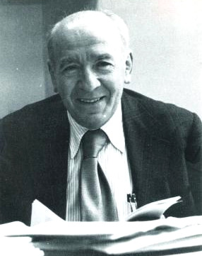
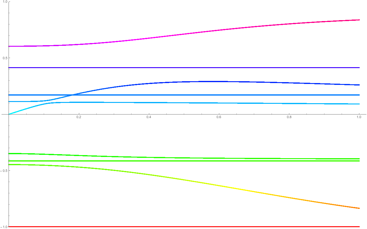
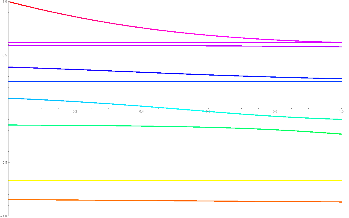
When adding a simplex $x$ to a complex we add a new row and column to the matrix $L$. We can look at the eigenvalues of $L(t)$, the matrix in which the new column and row are multiplied by $t$. What we see is that if x is even dimensional, then the new eigenvalue $\lambda_x(t)$ satisfies $\lambda_x(0)=0$ and $\lambda_x(t)>0$ for all $t >0, t \leq 1$. If $x$ is odd dimensional, we see that $\lambda_x(t)>0$ for $t \in (0,1/2)$ and $\lambda_x(t)<0$ for $t \in (1/2,1]$ and $\lambda_x(0)=\lambda_x(1/2)=0$. The fact that $\lambda_x(1/2)=0$ can be seen by giving an explicit eigenvector vector. If one can show that in the odd dimensional cell addition, only one eigenvalue crosses and in the even dimensional case, none crosses over when interpolating the Laplacians, then we would be done. Here are some typical pictures. We see the eigenvalues in the neighborhood of 0 only. In the first case, we add an even dimensional simplex to the CW complex. What happens is that a new eigenvalue is born and no eigenvalue crosses 0. In the second case, when we add an odd dimensional simplex to the CW complex, there is a new positive eigenvalue born, but this eigenvalue will cross 0 at the deformation parmeter t=1/2 exactly ending up on the other side, contributing one more negative eigenvalue. We know from the determinant story only that modulo 2, we have the right number of eigenvalues. In principle, it would be possible still that two eigenvalues cross the 0 level during the deformation from t=0 to t=1. It appears however that only for one value t=1/2, the Laplacian L(t) is possibly non-invertible and that this happens exactly if we add an odd dimensional simplex to the CW complex.
|
 |
At the moment, I believe it is not that impossible, maybe just technically a bit too complicated: one idea is just write the Reighleigh expressions for the derivatives of the eigenvalues when making a deformation which is standard perturbation theory of eigenvalues of self-adjoint matrices. Maybe one can say something about the second derivative. At that stage it is good to keep the eye open for a “raising sea” solution.
Zeta function
The zeta function of a simplicial complex $G$ with $n$ sets is the function
Note that this is an other zeta function than the Bowen Lanford zeta function discussed in this context
too. See the Handout.
It is important to know that there are three type of Zeta function classes (for any geometry!). This basic division brings a bit order in the zoo of zeta function (there are dozens!). What is exciting is that there these zeta functions come from different areas of mathematics and sometimes are related. Zeta functions are a bridge between different parts of mathematics!
| Spectral Zeta function | Dynamical Zeta function | Prime Zeta function |
| Examples: Riemann zeta function generalized to Minakshisundaram-Pleijel zeta function for manifolds, Zeta function of a graph |
Examples: Riemann zeta function, Artin-Mazur, Ihara, Bowen-Lanford generalized to Ruelle zeta function. |
Examples: Riemann Zeta function, Zeta functions to other number fields, L-functions. |
We are still experimenting. This is time consuming and will probably only be done later as there is little time during the semester.
- $\zeta(0)=\zeta(1)=n$.
- $\zeta(-1)$ is the sum $\sum_x 1-\chi(S(x))$.
- The values of $\zeta(n)$ for integer determines the law of the random variable. (moment problem)
- The zeta function determines the Euler characteristic of G.
- We have a two sided sequence of integers $r(n)= tr(L^n)$, where $n \in Z$ (integers!).
- We see a strong correlation between the minimum of the heat function tr(exp(-Lt)) and the dimension
- If $\zeta_{BL}(s) = 1/det(1-s A)$ is the Bowen-Lanford zeta function of the connection graph, then $det(L)=1/\zeta_{BL}(-1)$.
We also know that $\exp(\zeta'(0)) = 1/det(L)$. This is the common starting point to zeta-regularizations of determinants
in differential geometry. We see that there is at least one common thing between $\zeta_{BL}$ and $\zeta$.
Obvious questions are:
- What possible multiplicities of eigenvalues can occur?
- Is there a maybe obvious reconstruction of the complex from the eigenvalues? First, we would like to
reconstruct the complex from the eigenvalues and eigenvectors. - What is the significance of the maximal or minimal eigenvalue of L
- What is the significance of the maximal or minimal eigenvalue of g
- What is the significance of the minimum of tr(exp(-L t))?
- What is the significance of the roots of the zeta function?
- Can one read off the Betti numbers from the eigenvalues of L or the zeta function?
- Are there more relations between the spectral and dynamical zeta function $\zeta_{BL}(s)=1/det(1-sA)$?
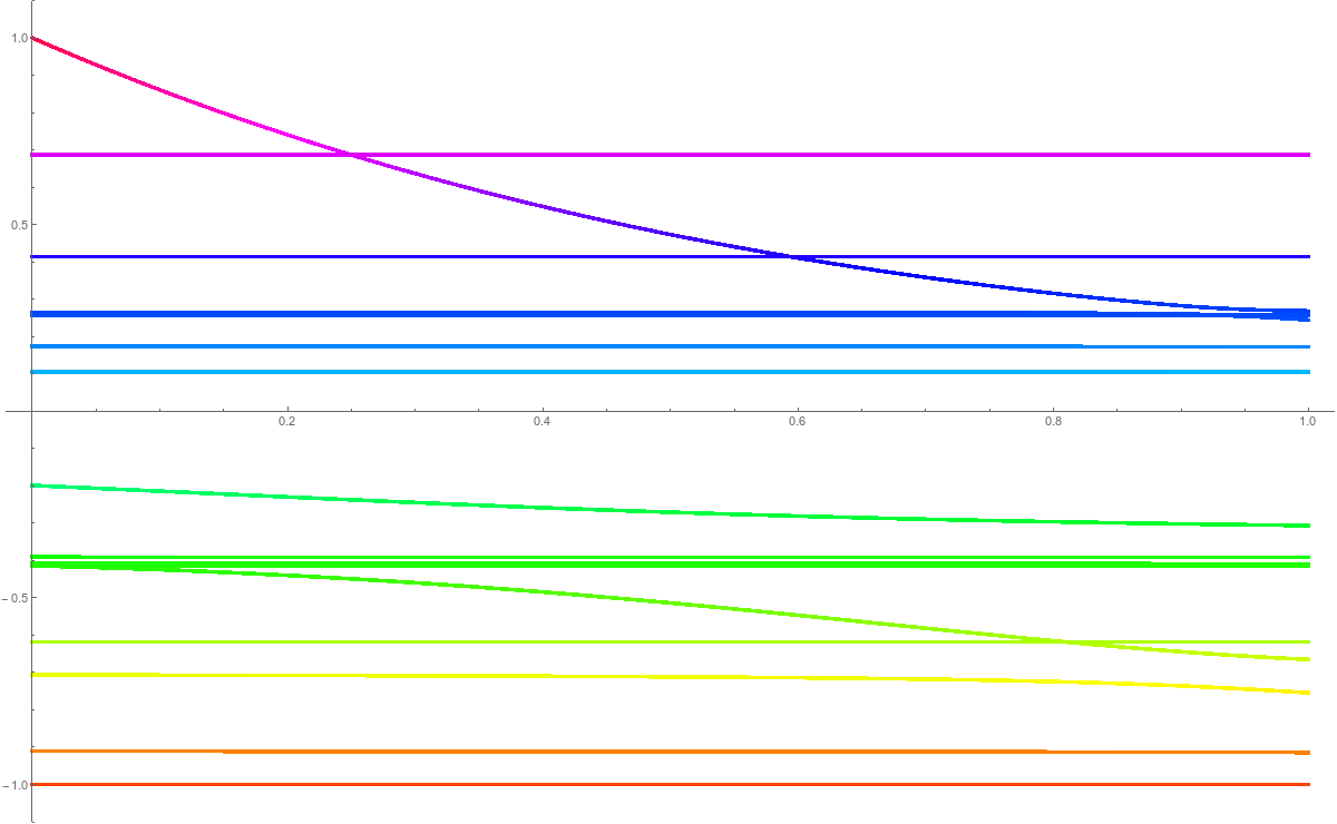
Update: 10/22/2017: 4 PM: during my run around the Mystic lakes, it occured to me that the deformation was not smart. Its just better to define L(t) by taking L but multiplying only the off diagonal entries of L in the last row by t. This has seems now to have a very nice effect: the multiplicative Poincare-Hopf formula det(L(G+x)) = det(L(G)) (1-X(S(x))) now becomes det(L(G+x)) = det(L(G)) (1-t X(S(x))). This explains why we have exactly one root at t=1/2 in the case when S(x) has Euler characteristic 2 and that we have no addition al root else. The proof in the general case is just Gabriel Cramer. Here are the eigenvalues seen in the new deformation picture
|
 |
And here is a picture of Gabriel Cramer:
October 23, 2017: a consequence of the formula $\chi(G)=B-F$ is $\chi(G) = (2/(\pi i)) tr(log(i L))$. This uses the unimodularlity theorem assuring that the real part of the trace of log(i L)) is zero. This rewriting again indicates that the Euler characteristic is an energy. It is here a logarithmic energy of the spectrum of iL. And it is a natural energy as in the complex plane (where the eigenvalues live), the logarithmic energy is the natural energy, the “Newton energy”.
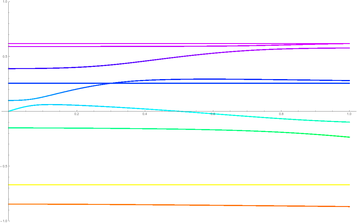
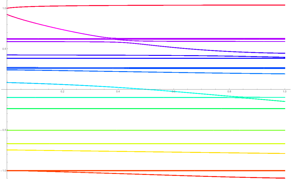
October 24, 2017: The one column deformation still needs to be studied more as we also want to understand the motion of the eigenvalues under the deformation The formula det(L(G+_t x)) = det(L(G)) (1-t X(S(x))) appears to be right under the deformation but how do the eigenvalues change? Most eigenvalues do not change very much. Here are two more examples of pretty random complexes. In the first case, an even dimensional simplex is added. In the second case, an odd dimensional simplex is added. The starting point is in both cases an eigenvalue 1. But it can be an other eigenvalue which travels linearly through 0.
 |
|