The Hamiltonian Manifold Theorem

The Hamiltonian manifold theorem

I recently finished proving a theorem in graph theory establishing that connected geometric networks which triangulate a manifold with or without boundary are Hamiltonian in the sense that they admit a Hamiltonian cycle. (This project got started already in 2014. I gave it a push in the late spring, early summer of 2018 and essentially finished it up in Switzerland. The first write-up is here on the ArXiv). In order to make the statement precise, one has to work with clear graph theoretical definitions of discrete manifolds. The inductive definition of these d-graphs and d-graphs with boundary is given below. It is the recursive nature of the definitions which make the result constructive. The theorem tells:

The result is a bit stronger. First of all, it is always possible to chose the Hamiltonian cycle so that it intersects a given maximal simplex in an edge. This is an important property as it allows to glue Hamiltonian cycles in different close connected components. Furthermore, the class of discrete manifolds can be extended a bit to what we call generalized d-graphs. We also see that the result is constructive and that the Hamiltonian cycle can be computed in in linear time, as is already known in dimension 2. For general graphs, it is well known that the computation of Hamiltonian paths is a prototype of a “hard problem”. The manifold structure tames the difficulty and renders the problem “easy”.

The result generalizes a result of Hassler Whitney from 1931, who proved a theorem implying that all 4-connected maximal planar graphs are Hamiltonian. But 4-connected maximal planar graphs are exactly the class of 2-spheres. Whitney’s result was later generalized by Bill Tutte and generalized to 4-connected planar graphs. We will see that the class of 2-dimensional graphs considered here go beyond Whitney as well as Tutte’s as we also have mainy non-planar and non-4-connected graphs covered by our condition.

Some slides (added June 21, 2018):

[Update June 21, 2018: in the stides, it was still claimed that one can find a Hamiltonian path visiting each facet. This is too strong and not needed. We need only to be able to get a Hamiltonian path visiting a fixed facet. It is no problem to upgrade from the statement with Hamiltonian to the statement with strong Hamiltonian property: given a facet x. If it is at the boundary, we can use induction already. If it is not at the boundary, cut a few edges so that it is at the boundary. The Hamiltonian cycle is now also a Hamiltonian cycle, when adding back the edges.

This argument is quite general. We can remove an arbitrary set of edges (as long as we stay in the class of generalized d-graphs), use the Hamiltonian property there and so have a Hamiltonian cycle which avoids the selected edges.

We never in the preprint proved that a Hamiltonian path can be found which hits all maximal simplices. We thought this to be obvious from the induction as all simplices are adjacent to a boundary simplex, after cutting things up. This is correct unti then. The problem is that after rerouting to reach the near boundary points, we detach some simplices from the boundary. At the moment, we don’t know whether one can always
force a Hamiltonian cycle to visit all maximal simplices. It is fortunatly not needed for the Hamiltonian manifold theorem. ]

Definitions

Definitions: a $d$-graph is a finite simple graph for which every unit sphere is a $(d-1)$-sphere. A $d$-sphere is $d$-graph such that removing one vertex renders the graph contractible. A graph is called contractible (*) if there exists a vertex for which the unit sphere and the graph without that vertex are both contractible. These inductive definitions are primed with the assumptions that the empty graph $0$ is the $(-1)$-sphere and that the one-point graph $1$ is contractible. A d-graph with boundary is a finite simple graph for which every unit sphere is either a (d-1) sphere or a (d-1) ball. A d-ball is a d-sphere with one vertex taken away. A finite simple graph $G$ is Hamiltonian, if there is a closed cycle in $G$ which visits every vertex exactly once.

(*) we use contractible in what is sometimes called collapsible and would call graphs homotopic to 1 simply “homotopic to 1”. In most cases this distinction is irrelevant but also in the discrete cases like the Bing house or dunce hat require to distinguish this.

Examples

• the empty graph is the (-1)-sphere, the 1-point graph is the 1-ball, the 2 point graph 2 is the 0-sphere, the k-point graph k is a 0-graph. The path graph is a 1-graph with boundary. None of these are Hamiltonian except maybe 1, if we consider sitting at a point a “cycle”.
• the circular graph $C_n$ for $n \geq 4$ is a 1-sphere. It is Hamiltonian. The Hamiltonian path is the graph itself.
• the wheel graph $W_n$ for $n \geq 4$ is a 2-ball with boundary. The boundary is $C_n$. Also the Wheel graph is Hamiltonian.
• the octahedron and icosahedron are the two Platonic solids which are 2-spheres. The tetrahedron is a generalized 3-ball as defined below and the cube and dodecahedron are one dimensional graphs (but not 1-graphs). All platonic solids are Hamiltonian.
• the cube graph is the dual graph of the octahedron. Dual graphs of d-spheres are always 1-dimensional and Hamiltonian.
• the figure 8 graph is not a 1-graph as there is a unit sphere which is the $0$-graph $4$ consisting of 4 isolated points. It is not Hamiltonian.
• if G is a p-graph and H is a q-graph, then $G \times H$ [the graph for which the vertex set are the 2-tuples (x,y) of simplices and where two are connected if one is contained in the other], is a $(p+q)$-graph. For example, $C_n \times C_m$ is a 2-torus with $(2n) * (2m)$ vertices.
• if $G$ is a $p$-graph and H is a $q$-graph with boundary, then $G \times H$ is a $(p+q)$-graph with boundary. The product of a path graph $P_p$ with a circular graph $C_q$ for example is $P_p x C_q$ which is a discrete cylinder.
• if G is a p-graph with boundary and H is a q-graph with boundary, then P x Q is a $(p+q)$- graph with boundary. The product of two path graphs $P_q \times P_q$ for example is a discrete rectangle.
• if $G$ is a $d$-graph without boundary, then the cone extension $G \oplus 1$ is a (d+1)-graph with boundary $G$. The cone extension of a $d$-sphere $G$ is a $(d+1)$ ball.
• if $G$ is a p-graph without boundary, then the suspension $G \oplus 2$ is a $(p_1)$-graph without boundary. The octahedron for example is the suspension of $C_4$. The d-fold suspension $2 \oplus 2 \cdots \oplus 2$ of $2$ is a $d$-sphere.
• if $G,H$ are two discrete $2$-tori. Pick a vertex $x$ in $G$ and a vertex $y$ in $H$ such that $S(x)$ and $S(y)$ are isomorphic. Taking the disjoint union of $G-x$ and $H-y$ and identifying $S(x)$ with $S(y)$ produces a double torus, a genus $2$ surface. It is a connected sum of $G$ and $H$.
• if G is a d-graph with or without boundary and e=(a,b) is an interior edge meaning $S=S(a) \cap S(b)$ is a $(d-2)$ dimensional sphere, then adding a new vertex on $e$ and connecting it to $S$ is an edge subdivision. One can get back $G$ by an edge collapse of either $ac$ or $bc$.
• if G is a d-ball and $H=G+_B x$ is a cone construction over the unit ball $B=B(y) \cap \delta G$ of a boundary point $y \in \delta G$, then $H$ is a d-ball. Doing an edge collapse of the interior edge e=(x,y) in H gives back $G$.

Enemies of Hamiltonian

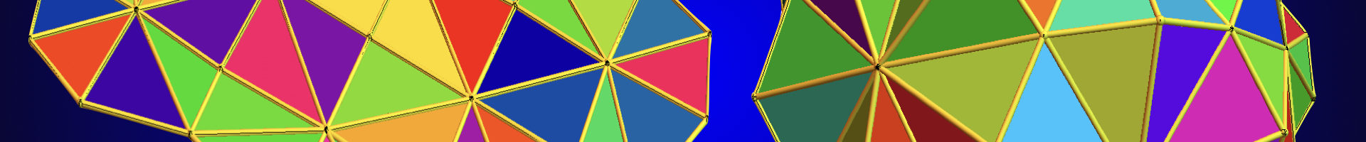
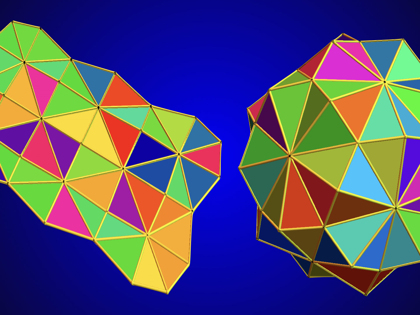
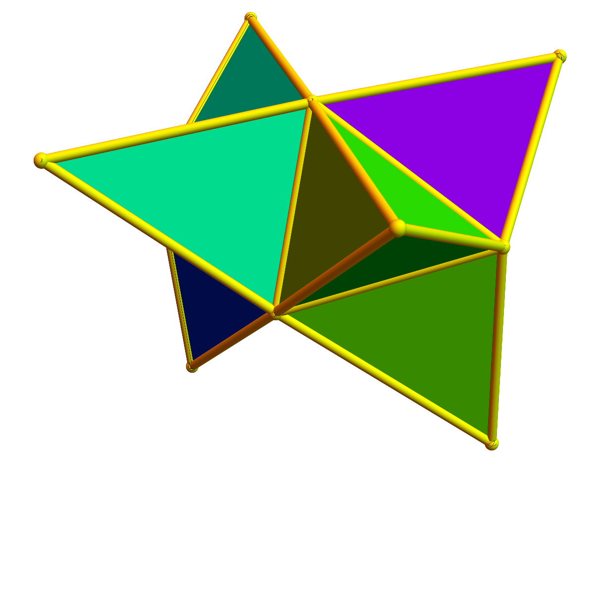
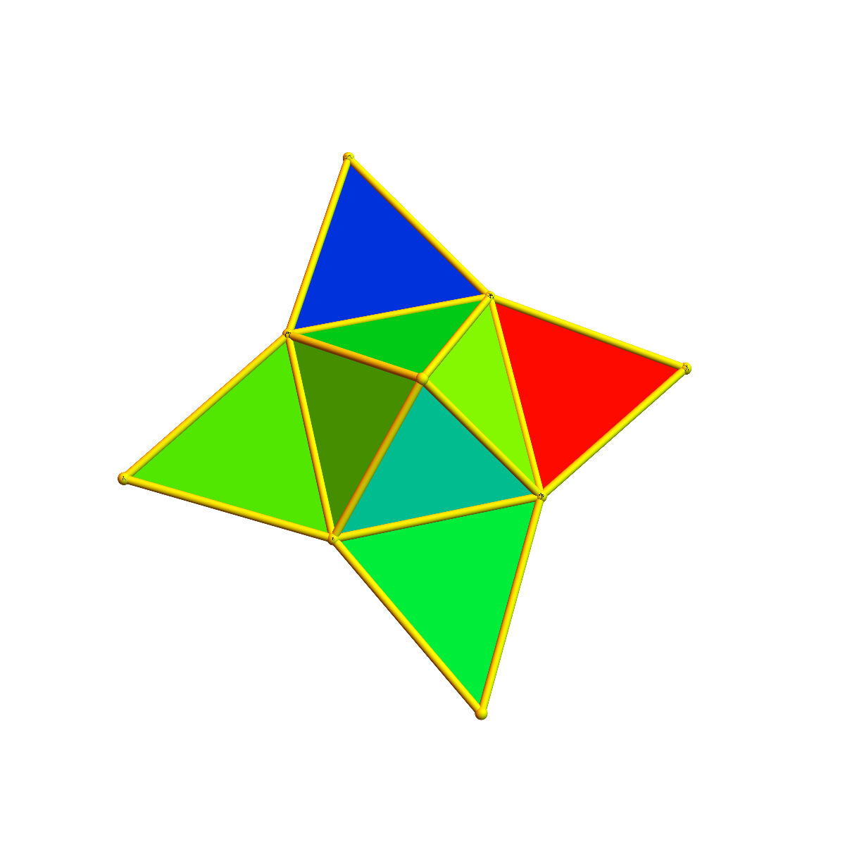
Here are two important examples of graphs which are both close to the class of graphs for which we prove the theorem but which are both not Hamiltonian. The first is the Goldner-Harary graph which looks a bit like a 3-ball but fails the property of being a generalized 3-graph. The second example is the stellated square graph, which look a bit like a 2-ball but in which the spikes shield the central point away from being reachable.

Generalized objects

When proving the result, it is convenient to look at slightly larger class of d-graphs with or without boundary.

Definition: a finite simple graph is generalized $d$-graph with boundary, if every unit sphere is either a (d-1)-sphere, a (d-1) ball or a (d-1) simplex.
In dimension d=2, not all these graphs are Hamiltonian. Examples are stellated wheel graphs in two dimensions. What we need is to have:

Definition: a generalized d-graph has an accessible boundary, if every interior vertex near the boundary has a unit sphere which intersects the boundary in a graph which contains an edge. In dimension d larger than 2, we only need the local sphere condition.

The triangle graph $K_3$ for example is a simplex and not a 2-ball as the unit spheres are not spheres. It is a generalized 2-ball. The diamond graph obtained by attaching two triangles along an edge is also not a 2-graph with boundary because for two vertices the unit sphere is $K_2$ and not a 1-ball as needed for a 2-ball. Also the Avici graph, obtained by gluing two tetrahedra together along a triangle is not a 3-ball but a generalized 3-ball. We need the limiting cases because we will remove interior vertices. The Goldner Harary graph obtained by stellate each of the 6 exterior faces of the Avici graph is not a generalized 3-ball because some unit spheres are neither 2-balls, nor 2-simplices nor 2-spheres. An other important prototype example is the stellated wheel graph, which fails the inner sphere property. It is not Hamiltonian. Also the stellated octahedron is not Hamiltonian. It also has an isolated inner sphere.

The Swiss Cheese proof

The proof is explicit and constructive. We can cut up the $d$-graph recursively by cutting holes, building cavities from the boundary and then roughing up the boundary to reach all interior points, then we have achieved that the graph becomes a $(d-1)$-graph without boundary.

There is only a bit of a pickle with isolated inaccessible inner parts in dimension 2. We can bypass this by enlarging the holes slightly. We could also refer to the literature and cite that Whitney’s theorem is now known to be stronger: 4-connected maximal planar graphs are also Hamiltonian connected implying that we can force a Hamiltonian path to go through a prescribed edge.

Cutting holes

Given a $d$ graph $G$ with or without boundary. Lets us call an interior vertex a very interior point if its geodesic distance to the boundary is 2 or more. For such a point $x$, we can isolate the ball $B(x)$ from the rest, ignoring all the connections from $B(x)$ to the rest of the graph $G$ except for a bridge going from $B(x)$ to the rest. This surgery preserves the class of $d$-graphs with boundary.

Building bridges

Given two separated boundary parts of a d-graph. Assume one has a face $x$ and the other has a face $y$, which build a prism allow to join Hamiltonian paths. When excluding the interior of this prism, we end up with a larger connected boundary part. By building caves and joining them with bridges, we end up eventually with a d-graph which has no very interior inner points any more.

Edging the boundary

We can reach boundary points by either removing a vertex with its connections from the boundary, preserving the d-graph property, or then by just carving in a small cut, taking an edge and detouring it to an interior point. In dimensions d larger than 2, every interior point near the boundary can be reached by small cuts because the intersection of two neighboring unit spheres is d-2 dimensional which for d larger than 2 has some edges.

Proof

The proof goes by induction with respect to dimension. The induction assumption is the case d=1, where we know that all connected 1-graphs without boundary are Hamiltonian. Now take a d-graph $G$ with boundary. If there is an interior vertex for which the unit sphere $S(x)$ does not intersect the boundary of $G$, build a prismatic bridge between $B(x)$ and $G-B(x)$, and combine the Hamiltonian paths in $B(x)$ and $G-B(x))$. To establish the Hamiltonian property in $G$, one therefore only needs to establish it for $G-B(x)$. Proceed so with all interior points of distance $2$ or more to the boundary. Then we cave out boundary points which are in distance 2 or more to an other boundary. Now reduce one by one the interior points with distance 1 to the boundary by cutting a $(d-1)$ prismatic hole into the boundary $\delta G$ exposing the point nearby. As cutting the holes does change the vertex set the Hamiltonian property of the graph does not change. Finally, once we reach the situation without interior point, we actually deal with a (d-1) graph with boundary. Each boundary component is Hamiltonian. Now connect the boundary components with prismatic bridges.

The algorithm

Lets call $C(G)$ a Hamiltonian cycle for a connected d-graph $G$:

1. If a boundary $\delta G$ is available, identity the vertices of the subgraph $\delta G$. It can be the empty set if the graph has no boundary.
2. Find an interior point $x$ in distance $2$ from the boundary $\delta G$. Remove $x$ from $G$ and join the unit sphere $S(x)$ to the boundary $\delta G$. Find a Hamiltonian cycle in the unit ball $B(x)$. Build a bridge from $S(x)$ to $\delta G$ using a pyramid. Now we have a new generalized $d$-ball with boundary. Repeat this step 2) until no interior points of distance 2 to the boundary can be found any more.
3. If we should end up with an interior point $y$ in distance $1$ to the boundary which is “boxed in” in the sense that its unit sphere $S(y)$ has no edge in common with $\delta G$, we make the interior of one of the neighboring holes larger to absorb some point $z \in S(y)$, allowing $y$ to be reached. This case only can occur in dimension $2$ because for $d \geq 2$, the intersection of two neighboring spheres in $\delta G$ has positive dimension and so contains an edge.
4. Now we have have a graph for which every still remaining interior point can be reached from the boundary. Build Hamiltonian cycle in each of the connected components of the boundary and connect them with bridges. This cycle covers now everything except the interior points in distance $1$ from the boundary.
5. Find an interior point $x$ in distance 1 from the boundary. Build a detour so have that interior point is included into the Hamiltonian path. Continue with step 5) until no interior points are available any more. Now we have a Hamiltonian cycle in the entire graph.