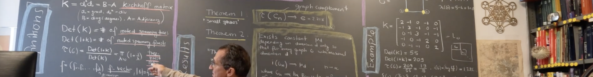
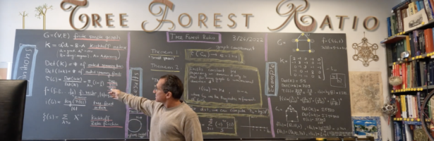
Tree Forest Ratio - Quantum Calculus

The tree forest ratio of a finite simple graph is the number of rooted spanning forests divided by the number of rooted spanning trees. By the Kirchhoff matrix tree theorem and the Chebotarev-Shamis matrix forest theorem this is $\tau = Det(1+K)/Det(K)$ where Det is the pseudo determinant and K the Kirchhoff matrix the ratio is $\prod_{\lambda>0} (1+\frac{1}{\lambda})$ , where $\lambda$ runs over all non-zero eigenvalues of K. We also have $\log(\tau) = \sum_{s=1}^{\infty} (-1)^{k+1} \zeta(s)/s$ , where $\zeta(s)=\sum_{\lambda>0} \lambda^{-s}$ is the spectral zeta function of the graph. For the complete graph $K_n$ for example, we have $\tau = (1+1/n)^{n-1}$ which converges to $e$ in the limit $n \to \infty$ . This is quite robust for very small graphs like complements of circular graphs. In general $\tau$ is huge. Our main result is that the tree forest index $i(G_n) = \log(\tau(G_n))/|G_n|$ converges in the limit $n \to \infty$ to a constant which only depends on the maximal dimension of G. In the case d=1, the limit is $\log(\phi^2)$ , where $\phi$ is the golden ratio. The proof of our theorem is even simpler than the spectral universality result from a couple of years ago which assured that the density of states of $G_n$ converged weakly in a universal way. Also there, the one dimensional case was explicit. Here we have just to note that the Barycentric limit is actually the Barycentric limit of the forests as $\log(T(G_n))$ (the tree index) grows much slower than $\log(F(G_n))$ (the forest index), then note that $\log(F(A+B)) = \log(F(A)) + \log(F(B))$ for disjoint union A+B, and finally that the Barycentric refined simplex can be decomposed into $(d+1)!$ smaller simplices which intersect in boundary parts of smaller dimension. The growth rate of trees or forests in different dimensions is stratified by dimension. This can be used to show that $\log(F(G_n))/|G_n|$ is a Cauchy sequence. In each step we add an error term which is getting exponentially smaller with n.

Update of March 31, 2022: today, while running early afternoon through Brighton, I realized that there could be a more elegant proof of convergence which uses the already known Barycentral spectral universality. The later tells that the eigenvalue list, when indexed on the interval [0,1] converges to a measure which only depends on dimension. Now look at $\frac{1}{n} \log (\tau(G)) = \frac{1}{n} \sum_{k=1}^n \log(1+\lambda_k^{-1})$ which converges to a potential theoretical energy $\int_{\mathbb{R}} \log(1+z) d\mu(z)$ , where $\mu$ is the measure pulled back by $f(z)=1/z$ . Now, if $G_n$ are the Barycentric refinements, then the number of vertices (and so the number of eigenvalues) is smaller than the number of simplices (the volume) but it is comparable as the number of vertices in $G_{n+1}$ is the total number of simplices in $G_n$ and so larger. So, dividing by the number of simplices or the number of vertices does not matter. We do not want to modify the definition of the tree forest index as we want still to get that for complete graphs, the limit is e. In that case we have seen that the tree forest ratio is $(1+1/n)^{n-1} \to e$ so that the tree forest index is 1 in the limit of the graph sequence $K_n$ . The limit e can also be explained by determinants and Fredholm determinants and the ration of the number of permutations versus the number of derangements (fixed point free permutations). I pointed this out in this article from 2013. [By the way, in the first submission of July 15th 2013, I had not been aware yet of the Chebotarev-Shamis result. Still, that relation to the generalized Cauchy Binet theorem is a “proof from the book” as the proof could be given even in the abstract of the generalized Cauchy Binet formula. My tree forest article by the way starts with a cool voting interpretation of the forest number. ] Back to the convergence of the logarithmic energy: while for measures of compact support the logarithmic energy outside the support of the spectrum is no problem, we have here a measure $\mu$ that has not compact support. It amounts to estimate how thin the measure gets at infinity which is equivalent to stating how fast the eigenvalues of K go to zero for large $G_n$ . In solid state physics, such problems are well studied and related to tail behavior of the integrated density of states. This is related to the spectral gap= ground state the smallest non-zero eigenvalue of the graph. Of course, the tree forest ratio gives a direct bound on the ground state which is larger than $1/(\tau(G)-1)$ in full generality. This also gives directly a lower bound for the Cheeger constant $h(G)$ of the graph G which is $h(G) \geq 1/(\tau(G) - 1)$ but that is certainly a rough estimate. Still, it explains a bit why highly connected graphs like the complete graph have low tree forest ratio and large diameter networks (in comparison to the number of nodes) have large tree forest ratio. By the way, my numerical experiments strongly indicate the following conjecture which I do not know how to prove yet (or only show that this holds for perturbations of the graph meaning that we have a critical point but not necessarily a global maximum).

Conjecture: the graph with n vertices for which the tree forest ratio is maximal is the linear graph of length n-1. No other graph achieves this maximum.

The relation with the Cheeger constant definitely could be fleshed out more here. I learned a bit more about the Cheeger constant while refereeing last year a nice undergraduate senior thesis “Cheeger’s Inequality and its applications to the estimation of Network Congestion” by Christina Tran at the Harvard College. Christina had worked there mainly with the San Diego Laplacian (named so after Fan Chung who wrote a book on spectral graph theory using mostly that Laplacian) and not the Kirchhoff Laplacian. The San Diego Laplacian is well suited especially in Markov chain or other probabilistic set-ups. The Kirchhoff Laplacian is nice because it is mathematically closer to the Laplacian we have in calculus, because it is the zero’th block of the Hodge Laplacian, and because of the tree and forest theorems. In matters of the Cheeger constant, the connections with the smallest eigenvalue are essentially the same.

Author: oliverknill