
The strong ring of simplicial complexes
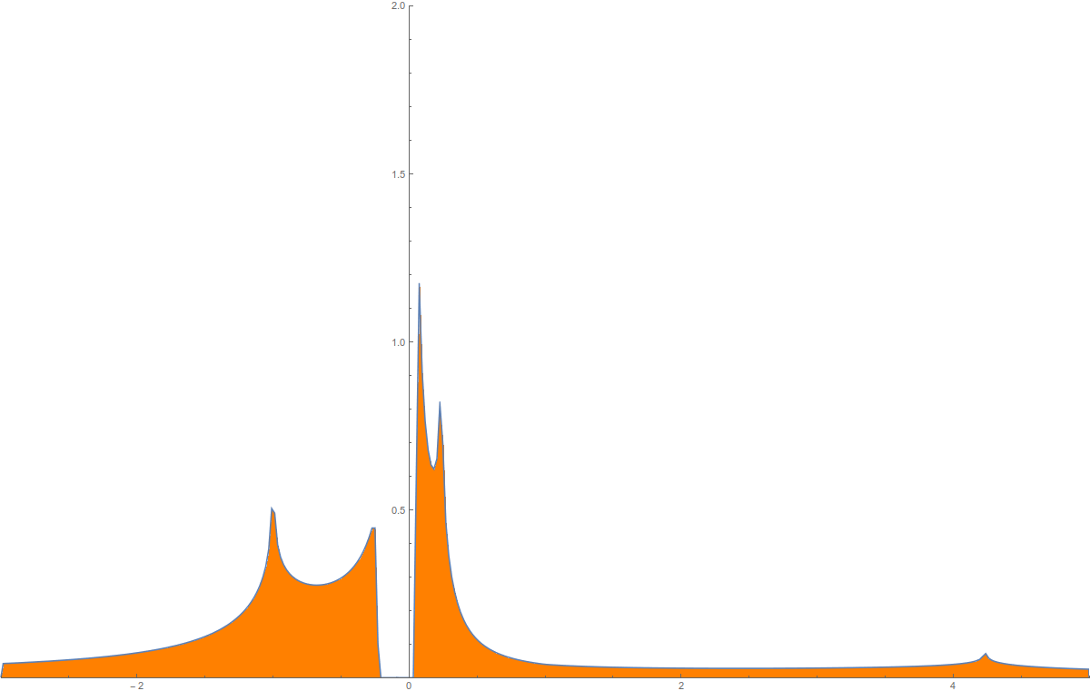
Update of August 5: the note “The Strong ring of Simplicial complexes” is out. It is a small step but I’m really happy with that structure as it helps to compute. Unlike in this post, also some Wu characteristic generalizations are added as these combinatorial invariants produce natural ring homomorphisms. Also interaction cohomology works well on the ring. There is also a picture of the density of states of the limiting connection operator of the lattice Z2, where we have a mass gap [-0.04,0.04].
What is the strong ring?
The strong ring of simplicial complexes is a cartesian closed category which is also a ring in a natural way. It is interesting topologically as there is a natural “geometric realisation” functor which maps a ring element into a topological space such that the product becomes the Cartesian product of topological spaces and the addition becomes the disjoint union. There are many categories which are also rings most notably the ring of sets with symmetric product as addition and intersection as multiplication. In the strong ring of simplicial complexes, the addition is the disjoint union and the multiplication is the cartesian product. [A simplicial complex is here understood a finite set of non-empty sets which is closed under the operation of taking finite non-empty subsets. As a finite set of sets, we can form the cartesian product G x H. But this cartesian product is no more a simplicial complex. It would be better to say the “strong ring generated by simplicial complexes” but we abbreviate it as “strong ring of simplicial complexes” for brevity.] Why is this ring interesting? The reason is that we can extend many results in topology to this ring. One is Hodge theory, relating linear algebra with cohomology, the second is potential theory, relating potential with curvature. And then there is algebra. The ring can be realized algebraically as a subring of the full Stanley Reisner ring. Every element in the ring can also be respresented as a signed graph in the Sabidussi ring of graphs. Both pictures are useful. The Stanley Reisner representation is useful to do computations purely algebraically using polynomials. The Sabidussi ring picture immediately gives the fundamental theorem of arithmetic in the strong ring. The additive primes are the connected components, the multiplicative primes are the connected simplicial complexes. Every additive prime has a unique prime factorization. The most spectacular display of the power of the ring is that we can associate to every element G two operators D and L. Both are matrices of the same size n, if G has n cells. The Dirac operator D has the property that the Hodge operator D*D =H reveals a complete picture about cohomology. The kernels of the Hodge blocks produce the cohomology groups and their dimension are the Betti numbers. The proof of Kuenneth is now easier as we have a concrete implementation of eigenfunctions relating them to eigenfunctions in the components. The connection operator L has the remarkable property that it is always invertible. This unimodularity result implies that the inverse matrix is integer valued where the entries can be interpreted as curature, indices or potential values depending on preference. But this is not all. There is a nice and natural compatibility between the spectra of D and L and arithmetic. The product of two ring elements produces a sum of the spectra of H and a product of spectra of L! The first property is known for the Laplacians in the continuum, connection Laplacians do not exist in the continuum. They only manifest in the Barycentric limit but then they are 2-adic. The notion of Barycentric refinement has the property that the first Barycentric refinement G1 is signed graph. This can be iterated and the Barycentric limit theorem assures that on a spectral level we have universality. Then there is what we call “strong Barycentric refinement”: if G=A x B is a product, we look at G1 = A1 x B1 and the sequence of Barycentric refinements Gn = An x Bn. We can thus form the Barycentric limit Zv, which has more structure than the usual lattice as it leads to almost periodic operators in the limit. The connection operator L stays invertible in the limit. This mass gap in an infinite volume limit makes many continuation results trivial as we just need the weak implicit function theorem. Here we see a big difference between the Dirac operator related to cohomology and the connection operator related to potential theory. The connection operator stays finite. Finally there are fine nonlinear integrable Hamiltonian systems associated to D and L. For D we can look at the isospectral deformations which is a Lax system. For L, we can for any functional look at the nonlinear Schroedinger evolution a natural choice being the Helmholtz Hamiltonian which is a sum of energy and entropy. Both quantities are natural as they are essentially unique when asking for quantities which are compatible with the arithmetic of the ring. An other interesting connection is that the dual to the Sabidussi ring is the Zykov ring in which the addition is the Zykov addition.
Representing ring elements
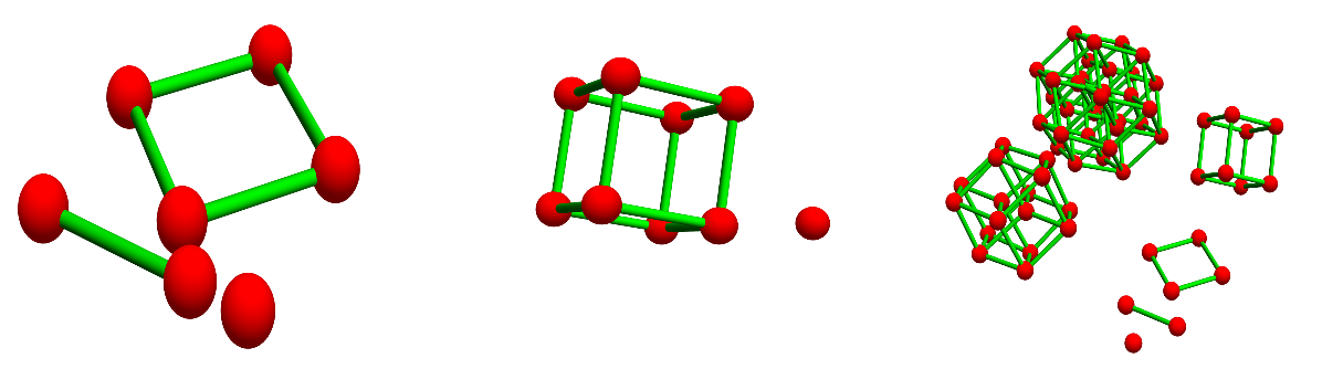
| Lets look at a concrete example of a ring element. It is the ring element G = C4 – 2 K3 + L2 x L3. It is the sum of three objects. The first, C4 is the discrete circle. The second -2 K3 is represented as two negative K3 complexes. What is the negative of a simplicial complex? Its just obtained as a natural extension from the additive monoid to a group. We are all well aware of this when introducing negative numbers or fractions. It was Grothendieck who formulated this idea in full generality. The third element is the product of two linear graphs. It represents a rectangle. But it is not given as a simplicial complex. In some sense, we have to think about the holes being filled with cells. In other words, the element L2 x L3 could naturally be though of as a discrete CW complex. |
|
In the discrete, the Whitehead concept of CW complex is done in the same way as in the continuum. It is a recursive conctruction in which new cells (contractible objects) are glued in along boundaries which are “spheres”. To define this propertly without geometric realisation, one has to define what a discrete sphere is but this can be done elegantly by asking a sphere to be an object for which every unit sphere is a sphere and for which removing one cell makes the remaining cell complex comtractible. CW complexes are natural and nice but they have one big deficit: they don’t play well along when looking at products. Intuitively what happens when we think about a CW complex, then we see an organically grown plant in which a time component, the growth of the plant is built in. When taking the product of two such plants, there is no linear way any more to tell how to attach cells. It just does not work and the best way to see that it does not work in a combinatorial setup is that it does not work in the continuum: CW complexes do not form a Cartesian closed category. The strong ring does form a combinatorical closed category however. It is a combinatorial category however in the sense that every ring element can be represented in a finite way. It is a category which a finitist can live and work with as nowhere in the construction, infinity is assumed. Of course, as logicians like Edward Nelson have pointed out, there is a “potential infinite” involved as we do not impose bound on the size of the complexes being built. But thats like looking at the set of integers. There is no infinity involved. We just refuse to impose a bound on the size of integers we use.
The ring element G of the strong ring can also be represented well as an algebraic object f=a+a b+b+b c+c+c d+d+a d-2(x+y+z+x y+x z+y z)+(u+u v+v)(p+p q+q+q r+r) in the full Stanley-Reisner ring. [ We say full Stanley-Reisner ring as Stanley-Reisner rings are usually finite rings associated to a finite simplicial complex.] The full Stanley-Reisner ring is a subring of the quotient ring of the ring Z[a,b,c,….], where we have infinitely many variables. Every element in the ring however is a finite sum of monomials and so has only finitely many variables. ] Writing the strong ring as a subring of the Stanley-Reisner ring is a bit similar as representing the ring of Gaussian integers as a subring of GL(2,Z). One has then piece of mind in that one knows what the square root of -1 is: it is just the matrix element which belongs to a rotation by 90 degrees. What about the elemnt -G if G is a simplicial complex? Yes, thousands of years ago, when the concept of negative numbers did not exist, one calculated with pebbles, three pebbles represent the number 3. The concept of -3, three negative pebbles came only later, maybe through the need to represent “debth” rather than “fortune”. Introducting negative simplicial complexes in the zero dimensional case is nothing else. We just label each simplicial complex appearing in a ring element with a sign and use identies like (-G) x (-K) = G x K which follow from the ring axioms.
The subring of zero dimensional elements in the strong ring is nothing else than the ring of integers. Numbers are represented by so as “pebbles’ = zero dimensional simplicial complexes or “finite sets”, which can be positive and negative. If a positive and negative pebble coexist, then one can let them “merge” and “annihilate” each other. Already the concept of integers involves so to speak that one looks at equivalence classes of pebbles. In the case of simplicial complexes, the equivalence relation is cast a bit wider: If we look at at a ring element G and see two connected components which are isomorphic as simplicial complexes and have opposite sign, we can delete them. That is the equivalence relation which is built in to the Stanley-Reisner ring. Mathematically, we look at a quotient ring of a subring of the ring Z[a,b,c,….]. We need to take a subring as the element 1 in the algebraic ring Z[a,b,c,…] is not there. The zero element in the ring is the empty complex and the one element in the ring is K1. The full Stanley-Reisner ring does not contain elements like 1+a as the algrebraic 1 in the polynomial ring is not considered in the Stanley-Reisner ring. The one-element in the ring is K1, a single pebble. What we mean with 2 G is that we have G + G or P2 x G, where P2 = K1 + K1 is the two point graph without edges.
|
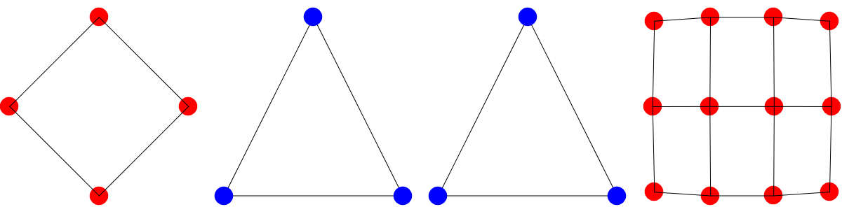
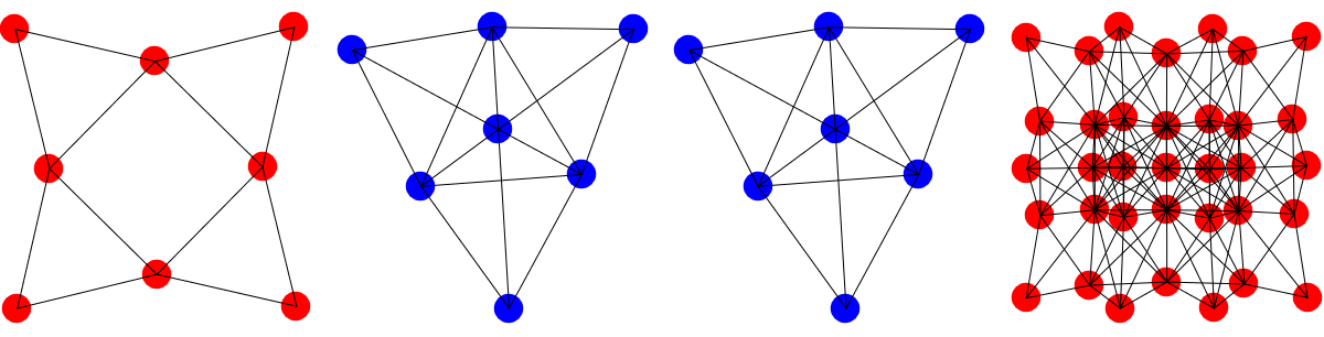
There are other ways to represent the element G. One is the signed Barycentric refinemen G1 of G. The other graph is the signed connection graph G’. Both graphs G1 and G have the same vertex set.
In G1 (seen to the right in the picture above), two elements are connected if one is contained in the other. The Barycentric refinement of C4 for example is C8. For G’ (we see to the right this graph) two elements are connected if they intersect. The connection graph of C4 already has triangles as two adjacent edges and its intersection point all intersect each other. If G is a complex, the connection graph is often homotopic to G but not always. For the octahedron graph, a 2-sphere, the connection graph is homotopic to a 3-sphere already. But this is because the octahedron was too small. If we look at G1 then then connection graph G1‘ is always homotopic to G1. Doing a Barycentric refinement is a bit like doing a regularization, clearing out pathologies which might be present still due to smallnes. The Barycentric refinement goes well with dimension, homotopy and cohomology and stabalizes most pathologies. |
|
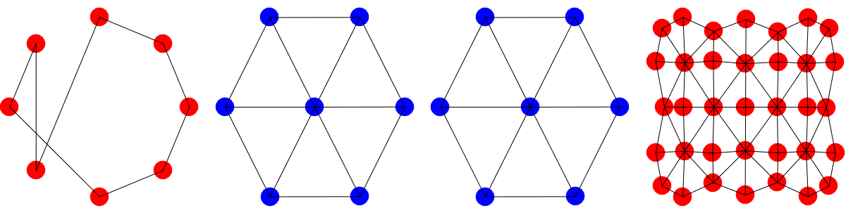
We have proven for example that after one Barycentric refinement the set of topologies which appear as unit spheres is fixed. It does not change any more under further Barycentric refinements but obviously there can be dramatic changes when doing the first Barycentric refinement. The triangle for example has no vertex with unit sphere which is not contractible. After one Barycentric refinement, the central vertex has a unit sphere (C6) which is not contractible. In some sense, the triangle is not a good picture of a disk as it is too small. The Barycentric refinement, the wheel graph however represents a “disc” very well. It has all the topological properties we expect from it. There are boundary elements, where the unit sphere is contractible and there are interior elements, where the unit sphere is not contractible.