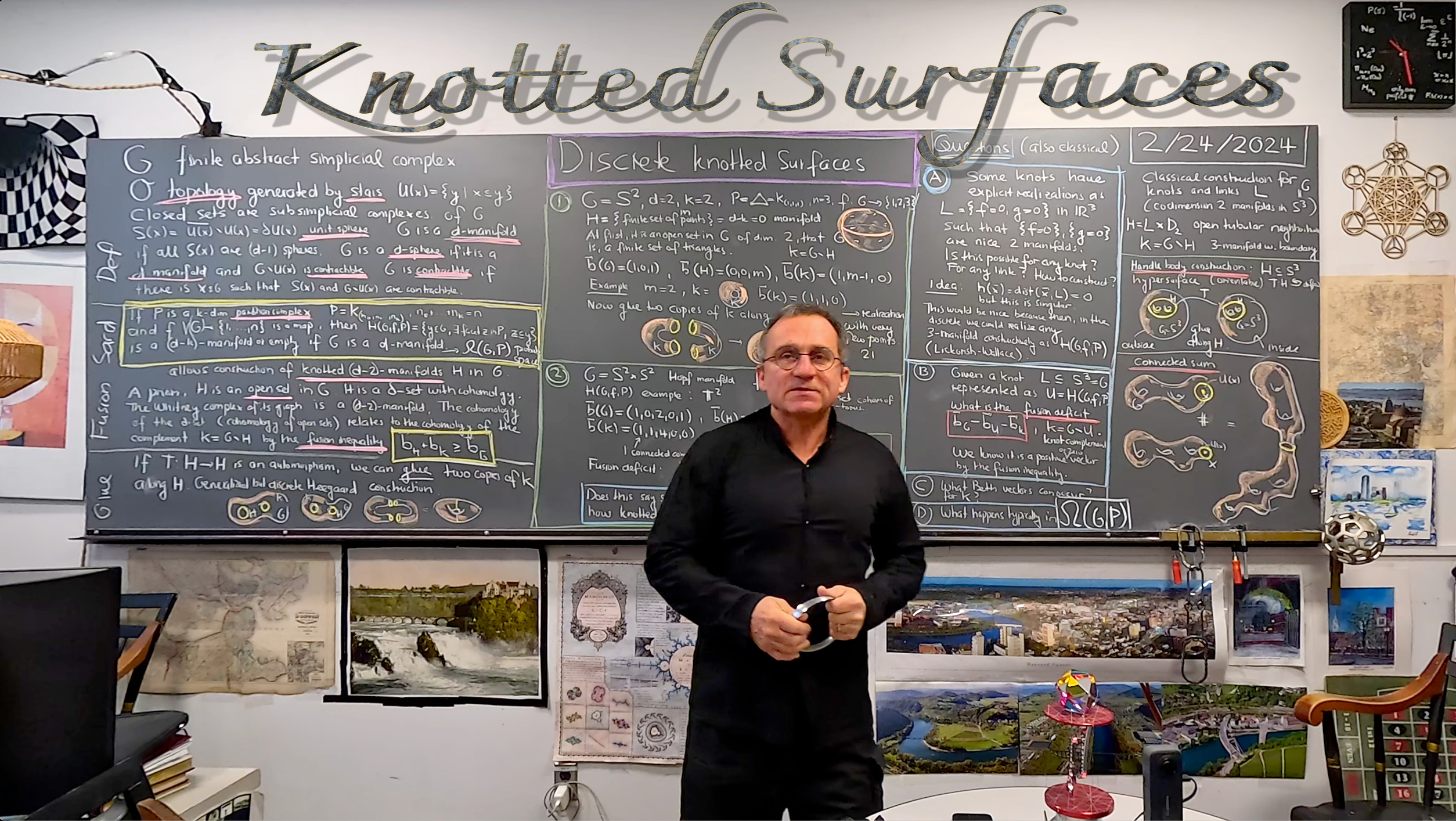
Discrete Knotted Surfaces - Quantum Calculus

If G is a d-manifold and $f:V(G) \to {1,2,3}$ is an arbitrary map, the discrete Sard theorem tells that $H=\{y, x \subset y\}$ is an open set in G that is a (d-k)-manifold. We mean with that the graph encoding the incidence of the sets in H is a (d-k) manifold. The sub-manifold H of K is in general knotted. A knotted 2-torus for example in $S^4$ would be an embedding of $T^2$ in $S^4$ that is not homotopic to the standard flat Clifford embedding of the 2-torus in $S^4$ . I’m excited about the discrete setup because it is a field of experimentation, where we can explicitly look at simplicial complexes within a given simplicial complex. Not that I have not tried before like in the case of knots with the picture seen to the right (JPG). But this was relatively hard to generate. I needed first of all to generate a suitable ambient space (3 dimensional triangulated lattice), then build by hand a polygon that would represent the knot and then implement it. When doing this by hand, we have to be careful for example that we have no self intersection of the curve. I did that by drawing a polygon on a square tiled paper decide about the upcrossings and downcrossings and implement that as hight. Unlike in the continuum where self-intersections happen with probability zero, in the discrete this is real. The nice thing about the Sard theorem is in the discrete that self-intersections never happen. The discrete world does not know singularities! Does not know singular varieties. Everything is given by manifolds. The co-dimension k manifold in the k manifold is always a manifold, if it is not empty. What one can do now also in the discrete is to take such a situation, make two copies, then glue the two copies together along the submanifold. This produces new manifolds. In some sense it is universal as Lickorish-Wallace illustrates: every 3 manifold can be generated by gluing complements of links together by doing the gluing in some non-obvious way like applying a Dehn twist.

One of the simplest cases is if G is a 3-sphere. Then H is a link in G. The complement K=G-H is a closed set in the Alexandroff topology and so a simplicial complex. It is exactly what the knot complement is classically: in knot theory one takes the complement of an open tubular neighborhood of the knot or link which is a 3-manifold with boundary. Everything is exactly as in the continuum. For example, the topology of the knot complement determines the knot up to reflection. There is a bit more. The fusion inequality tells that $b(H) + b(K) \geq b(G)$ . In the case of a link with m components, we have b(G)=(1,0,0,1), b(H)=(0,0,m,m) (note the shift as triangles are the smallest dimensional objects) and b(K) = (1,m,m-1,0). The fundamental group would give more information than the Betti numbers but I don’t have written code to compute the fundamental group. It is certainly computationally harder as one has to find the isotopy classes of paths put them as generators, then find the analog of the Wirtinger presentation. Nice would be if there was like with cohomology a Hodge approach for computing homotopy groups but that is unlikely given the non-commutat ive nature of the fundamental group. What I’m also interested in are other invariants like Wu Betti numbers. It is a cohomology theory which is computationally harder to compute but still has a Hodge approach. Maybe I will talk about this an other time. Unlike Wu characteristic which for manifolds with boundary agrees with the Euler characteristic, the Wu Betti numbers can distinguish spaces that are not-homotopic like the cylinder and the Moebius strip. (I gave once a math table talk in 2016 about this. It is attached as an appendix to this document. Fact is that computing this so far works for me only for small cases but it might be already very interesting in the smallest interesting case, the case of co-dimension 2 surfaces in $S^3$ , aka links.

I actually wanted to talk first a bit more about the gluing thing. Let me just illustrate this (as in the talk) with a tiny story where we can see all the details. it is kind of a Mickey-Mouse version of the Lickorish-Wallace theorem illustrating that we can get all 2-manifolds by just gluing links in $S^2$ . Links in $S^2$ are co-dimension 2 manifolds in $S^2$ which is a finite set of isolated points which has to be even as is a finite union of 0-dimensional spheres. The tubular neighborhood now is a bunch of open disks and the “link complement” is a sphere with finitely many open holes removed. It is a 2-manifold with boundary. Gluing the boundary circles together in some way (pair the finite set of points up and decide about an orientation for each) and glue things together. From the classification of surfaces one can see that every oriented 2-manifold can be obtained like that. By having one orientation switched for the gluing one can even get the non-orientable cases like that. The gluing procedure already appears in the connected sum construction in topology: take two 2-manifolds, pick a point in each manifold, remove an open ball around each point then glue the boundaires together.

Now there is something which needs to be said: The Sard theorem gives for codimension 2 manifolds in a 2-manifold just a finite set of facets. They can even be adjacent. In order that the gluing works, we need the two triangles not to touch and also that the glued space is not too small. If we take an octahedron with 6 points and try to do the gluing, we get an object with 6+6-3=9 points. On a simplicial complex level this gives a 2-torus with 9 points (this is two small for a Whitney complex of a graph) but if we look at the graph from a complex, we take the Whitney complex where every triangle is a face. This is why I chose as an example the icosahedron complex, where we have nicely separated polar triangles. If two such icosahedra are taken and the gluing is done, we get a torus with 12+12-3 vertices. Lets see that construction in all its detail.

G=Whitney[PolyhedronData["Icosahedron", "Skeleton"]];

gives the complex

G={{1}, {2}, {3}, {4}, {5}, {6}, {7}, {8}, {9}, {10}, {11}, {12}, {1, 3}, 
 {1, 5}, {1, 6}, {1, 9}, {1, 10}, {2, 4}, {2, 7}, {2, 8}, {2, 11}, {2, 12}, 
 {3, 7}, {3, 8}, {3, 9}, {3, 10}, {4, 5}, {4, 6}, {4, 11}, {4, 12}, {5, 6}, 
 {5, 9}, {5, 11}, {6, 10}, {6, 12}, {7, 8}, {7, 9}, {7, 11}, {8, 10}, {8, 12}, 
 {9, 11}, {10, 12}, {1, 3, 9}, {1, 3, 10}, {1, 5, 6}, {1, 5, 9}, {1, 6, 10}, 
 {2, 4, 11}, {2, 4, 12}, {2, 7, 8}, {2, 7, 11}, {2, 8, 12}, {3, 7, 8}, 
 {3, 7, 9}, {3, 8, 10}, {4, 5, 6}, {4, 5, 11}, {4, 6, 12}, {5, 9, 11}, 
 {6, 10, 12}, {7, 9, 11}, {8, 10, 12}};

We now chose the two triangles {1,5,6} and {2,7,8}. They are separated enough that we can glue the boundaries. Here is the gluing done, very slowly with each step. Note that almost all (except the last line) of the following code works by itself without additional code. The Betti implementation needs a handful of Mathematica code and was given a couple of times here on this blog already like here: the 5 lines of cohomology. let me add it here too again so that the entire thing can just be copy pasted without any additional stuff: just copy paste the following lines into Mathematica and get the

F[G_]:=Module[{l=Map[Length,G]},If[G=={},{},Table[Sum[If[l[[j]]==k,1,0],{j,Length[l]}],{k,Max[l]}]]];
s[x_]:=Signature[x];L=Length;s[x_,y_]:=If[SubsetQ[x,y]&&(L[x]==L[y]+1),s[Prepend[y,Complement[x,y][[1]]]]*s[x],0];
Dirac[G_]:=Module[{f=F[G],b,d,n=Length[G]},b=Prepend[Table[Sum[f[[l]],{l,k}],{k,Length[f]}],0];
  d=Table[s[G[[i]],G[[j]]],{i,n},{j,n}]; {d+Transpose[d],b}];
Hodge[G_]:=Module[{Q,b,H},{Q,b}=Dirac[G];H=Q.Q;Table[Table[H[[b[[k]]+i,b[[k]]+j]],{i,b[[k+1]]-b[[k]]},
{j,b[[k+1]]-b[[k]]}],{k,Length[b]-1}]]; nu[A_]:=If[A=={},0,Length[NullSpace[A]]];Betti[G_]:=Map[nu,Hodge[G]];
G={{1}, {2}, {3}, {4}, {5}, {6}, {7}, {8}, {9}, {10}, {11}, {12}, {1, 3}, 
 {1, 5}, {1, 6}, {1, 9}, {1, 10}, {2, 4}, {2, 7}, {2, 8}, {2, 11}, {2, 12}, 
 {3, 7}, {3, 8}, {3, 9}, {3, 10}, {4, 5}, {4, 6}, {4, 11}, {4, 12}, {5, 6}, 
 {5, 9}, {5, 11}, {6, 10}, {6, 12}, {7, 8}, {7, 9}, {7, 11}, {8, 10}, {8, 12}, 
 {9, 11}, {10, 12}, {1, 3, 9}, {1, 3, 10}, {1, 5, 6}, {1, 5, 9}, {1, 6, 10}, 
 {2, 4, 11}, {2, 4, 12}, {2, 7, 8}, {2, 7, 11}, {2, 8, 12}, {3, 7, 8}, 
 {3, 7, 9}, {3, 8, 10}, {4, 5, 6}, {4, 5, 11}, {4, 6, 12}, {5, 9, 11}, 
 {6, 10, 12}, {7, 9, 11}, {8, 10, 12}};
H={{1, 5, 6}, {2, 7, 8}};
Ver[X_]:=Union[Flatten[X]];
V=Ver[G]; n=Max[V]; W=V+n+1;
G1=G; G2=G;  H1=H; H2=H;
f=Table[V[[k]]->W[[k]],{k,Length[V]}];
G2=G2 /. f; H1=H; H2=H /. f;
W1=Ver[H1]; W2=Ver[H2];
K1=Complement[G1,H1]; K2=Complement[G2,H2];
g=Table[W1[[k]]->W2[[k]],{k,Length[W1]}];
K1=K1 /. g;
GG=Union[K1,K2]; 
Betti[GG] 
Betti[G]

The result is {1,2,1} which means that we have indeed got a torus. We can quickly check that we have indeed a manifold and also compute the curvature:

UnitSphere[s_,v_]:=VertexDelete[NeighborhoodGraph[s,v],v];
UnitSpheres[s_]:=Module[{v=VertexList[s]},Table[UnitSphere[s,v[[k]]],{k,L[v]}]];
ToGraph[G_]:=UndirectedGraph[n=Length[G];Graph[Range[n],
  Select[Flatten[Table[k->l,{k,n},{l,k+1,n}],1],(SubsetQ[G[[#[[2]]]],G[[#[[1]]]]])&]]];
Curvature[s_,v_]:=Module[{u=F[Whitney[UnitSphere[s,v]]]},1+Sum[u[[k]]*(-1)^k/(k+1),{k,Length[u]}]];
Curvatures[s_]:=Module[{v=VertexList[s]},Table[Curvature[s,v[[k]]],{k,Length[v]}]];
Generate[A_]:=If[A=={},{},Sort[Delete[Union[Sort[Flatten[Map[Subsets,A],1]]],1]]];
Whitney[s_]:=Generate[FindClique[s,Infinity,All]];
BettiGraph[s_]:=Betti[Whitney[s]]; 
Union[Map[BettiGraph,UnitSpheres[ToGraph[GG]]]]
Curvatures[ToGraph[GG]]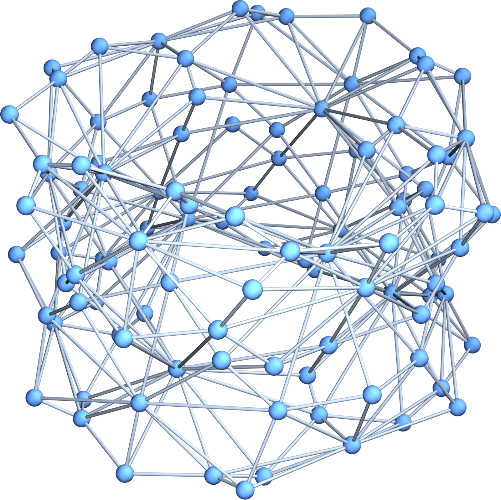

which confirms that every unit sphere in that graph is indeed a circular graph. We can look also at the curvatures for example. The graph of the complex has 54 vertices with curvature 1/3 and 36 vertices with zero curvature, there are 12 vertices with curvature -2/3 and 6 vertices with curvature -5/3. The total curvatur by Gauss-Bonnet is zero. Since the complex GG has 108 elements, the graph representing the torus has 108 elements. You see the graph to the right. It should be noted however how small the simplicial complex GG is. It is given here. Note that since both K1 and K2 are simplicial complexes also the glued version is a simplicial complex. The glued open sets H1 and H2 were both just unions of two stars: H1={{1, 5, 6}, {2, 7, 8}} and H2={{14, 18, 19}, {15, 20, 21}}; Both H1 and H2 are open sets in the Alexandrov topology and represent unions of two open disks. The gluing was done with the function g: {1 -> 14, 2 -> 15, 5 -> 18, 6 -> 19, 7 -> 20, 8 -> 21} which just renamed some of the vertices in the first icosahedron with the labels of the second icosahedron. It does not go easier than that.

GG={{3}, {4}, {9}, {10}, {11}, {12}, {14}, {15}, {16}, {17}, {18}, {19}, {20},
{21}, {22}, {23}, {24}, {25}, {3, 9}, {3, 10}, {3, 20}, {3, 21}, {4, 11},
{4, 12}, {4, 18}, {4, 19}, {9, 11}, {10, 12}, {14, 3}, {14, 9}, {14, 10},
{14, 16}, {14, 18}, {14, 19}, {14, 22}, {14, 23}, {15, 4}, {15, 11},
{15, 12}, {15, 17}, {15, 20}, {15, 21}, {15, 24}, {15, 25}, {16, 20},
{16, 21}, {16, 22}, {16, 23}, {17, 18}, {17, 19}, {17, 24}, {17, 25},
{18, 9}, {18, 11}, {18, 19}, {18, 22}, {18, 24}, {19, 10}, {19, 12},
{19, 23}, {19, 25}, {20, 9}, {20, 11}, {20, 21}, {20, 22}, {20, 24},
{21, 10}, {21, 12}, {21, 23}, {21, 25}, {22, 24}, {23, 25}, {3, 20, 9},
{3, 20, 21}, {3, 21, 10}, {4, 18, 11}, {4, 18, 19}, {4, 19, 12}, {14, 3, 9},
{14, 3, 10}, {14, 16, 22}, {14, 16, 23}, {14, 18, 9}, {14, 18, 22},
{14, 19, 10}, {14, 19, 23}, {15, 4, 11}, {15, 4, 12}, {15, 17, 24},
{15, 17, 25}, {15, 20, 11}, {15, 20, 24}, {15, 21, 12}, {15, 21, 25},
{16, 20, 21}, {16, 20, 22}, {16, 21, 23}, {17, 18, 19}, {17, 18, 24},
{17, 19, 25}, {18, 9, 11}, {18, 22, 24}, {19, 10, 12}, {19, 23, 25},
{20, 9, 11}, {20, 22, 24}, {21, 10, 12}, {21, 23, 25}}

Author: oliverknill