Here is some code illustrating the story. We take the 4 manifold 


,(-1,1),(1,-1),(1,1) \}")


[By the way, there are no any data which suggest that space is non-commutative (or discrete) in the very small. It is a speculation, similarly like the Demoktitus speculation who speculated that matter is discrete. Demokritus speculation should be considered flawed because he had based his observations on conclusions which have proven to be wrong (he must have noticed fine sand can not be crushed any more, which is of course wrong of the order by 4-5 orders of magnitudes. Serious experiments what matter and energy is came only more than 2000 years later especially with Lavoisier who started to understand some fundamental conservation principles of chemistry and could base it on experiments. We can in easily crush sand into molecules (by melting and evaporating it) or even atoms and the 20th century has shown 100 years after Lavoisier even beyond on the level of atoms). Modern speculations of the discreteness of space is based on having finite computable approximations like lattice gauge theory that can be used as a numerical method to compute things, say for Monte-Carlo simulations. Any numerical computation is a finite approximation. There is no evidence at all that space is discrete say on a level of 


Back to the non-commutatiivity I mentioned in the discrete. This is something we can talk about because everybody, can make the measurement and see it. Running computer code is doing an experiment. It is a priori only mathematics and not physics. Mathematical implementations of theories can be considered physical too. It is realized as an idea that can be written down with finitely many symbols and can be programmed with a finite program. It therefore exists. You can run the program bellow and see its output. It is just not necessarily part of the world which has been chosen to host us thinking about it. The physical world could only be a tiny part of what we can explore with our thoughts. In mathematics we can chose our axiom systems as we wish, provided of course that we do not run into an inconsistency. One of the reasons to think in finite mathematics is the possibility that any theory that includes the infinity axiom is fundamentally flawed and inconsistent. That is not impossible and Goedel has shown that we can within such a frame work not even prove consistency. It is a fundamental difficulty. When talking about finite sets only, we live less dangerously.
Here is the code:
Generate[A_]:=If[A=={},{},Sort[Delete[Union[Sort[Flatten[Map[Subsets,A],1]]],1]]];
Whitney[s_]:=Generate[FindClique[s,Infinity,All]];L=Length; Ver[X_]:=Union[Flatten[X]];
sig[x_]:=Signature[x]; nu[A_]:=If[A=={},0,L[NullSpace[A]]];       Rnd:=Random[]-1/2;
F[G_]:=Module[{l=Map[L,G]},If[G=={},{},Table[Sum[If[l[[j]]==k,1,0],{j,L[l]}],{k,Max[l]}]]];
sig[x_,y_]:=If[SubsetQ[x,y]&&(L[x]==L[y]+1),sig[Prepend[y,Complement[x,y][[1]]]]*sig[x],0];
Dirac[G_]:=Module[{f=F[G],b,d,n=L[G]},b=Prepend[Table[Sum[f[[l]],{l,k}],{k,L[f]}],0];
 d=Table[sig[G[[i]],G[[j]]],{i,n},{j,n}];{d+Transpose[d],b}];HH[G_]:=MatrixPower[Dirac[G][[1]],2];
Hodge[G_]:=Module[{Q,b,H},{Q,b}=Dirac[G];H=Q.Q;Table[Table[H[[b[[k]]+i,b[[k]]+j]],
 {i,b[[k+1]]-b[[k]]},{j,b[[k+1]]-b[[k]]}],{k,L[b]-1}]];
Betti[s_]:=Module[{G},If[GraphQ[s],G=Whitney[s],G=s];Map[nu,Hodge[G]]];
Facets[G_]:=Select[G,(L[#]==Max[Map[L,G]]) &];  Poly[X_]:=PolyhedronData[X,"Skeleton"];
RFunction[G_,P_]:=Module[{},R[x_]:=x->RandomChoice[Range[L[Ver[P]]]];Map[R,Ver[G]]];
RFunction[s_]:=Module[{G},If[GraphQ[s],G=Whitney[s],G=s];R[x_]:=x->Rnd;Map[R,Union[Flatten[G]]]];
AbstractSurface[G_,f_,A_]:=Select[G,(Sum[If[SubsetQ[#/.f,A[[l]]],1,0],{l,L[A]}]>0)&];
Z[n_]:=Partition[Range[n],1]; ZeroJoin[a_]:=If[L[a]==1,Z[a[[1]]],Whitney[CompleteGraph[a]]];
ToGraph[G_]:=UndirectedGraph[n=L[G];Graph[Range[n],
  Select[Flatten[Table[k->l,{k,n},{l,k+1,n}],1],(SubsetQ[G[[#[[2]]]],G[[#[[1]]]]])&]]];
S2xS2=Generate[{{1,2,3,4,6},{1,2,3,4,7},{1,2,3,6,9},{1,2,3,7,9},{1,2,4,5,8},{1,2,4,5,9},
  {1,2,4,6,8},{1,2,4,7,9},{1,2,5,6,8},{1,2,5,6,9},{1,3,4,6,7},{1,3,5,6,7},{1,3,5,6,9},
  {1,3,5,7,10},{1,3,5,9,11},{1,3,5,10,11},{1,3,7,9,10},{1,3,9,10,11},{1,4,5,8,10},
  {1,4,5,9,11},{1,4,5,10,11},{1,4,6,7,11},{1,4,6,8,10},{1,4,6,10,11},{1,4,7,9,11},
  {1,5,6,7,8},{1,5,7,8,10},{1,6,7,8,11},{1,6,8,10,11},{1,7,8,10,11},{1,7,9,10,11},
  {2,3,4,6,8},{2,3,4,7,8},{2,3,5,7,10},{2,3,5,7,11},{2,3,5,10,11},{2,3,6,8,10},{2,3,6,9,10},
  {2,3,7,8,11},{2,3,7,9,10},{2,3,8,10,11},{2,4,5,8,9},{2,4,7,8,9},{2,5,6,8,11},{2,5,6,9,10},
  {2,5,6,10,11},{2,5,7,8,9},{2,5,7,8,11},{2,5,7,9,10},{2,6,8,10,11},{3,4,6,7,11},{3,4,6,8,10},
  {3,4,6,9,10},{3,4,6,9,11},{3,4,7,8,11},{3,4,8,9,10},{3,4,8,9,11},{3,5,6,7,11},{3,5,6,9,11},
  {3,8,9,10,11},{4,5,6,9,10},{4,5,6,9,11},{4,5,6,10,11},{4,5,8,9,10},{4,7,8,9,11},{5,6,7,8,11},
  {5,7,8,9,10},{7,8,9,10,11}}];   P=ZeroJoin[{1,1,2}];P=P/.{1->3,2->4,3->1,4->2};
G=S2xS2;   V=Ver[P];   FF=Facets[P];   f=RFunction[G];     g=RFunction[G];
fg=Table[f[[k,1]]->(1+(Sign[f[[k,2]]]+1)+(Sign[g[[k,2]]]+1)/2),{k,Length[g]}];
gf=Table[f[[k,1]]->(1+(Sign[f[[k,2]]]+1)/2+(Sign[g[[k,2]]]+1)),{k,Length[g]}];
Hfg=AbstractSurface[G,fg,FF]; Hgf=AbstractSurface[G,gf,FF]; {Betti[Hfg],Betti[Hgf]}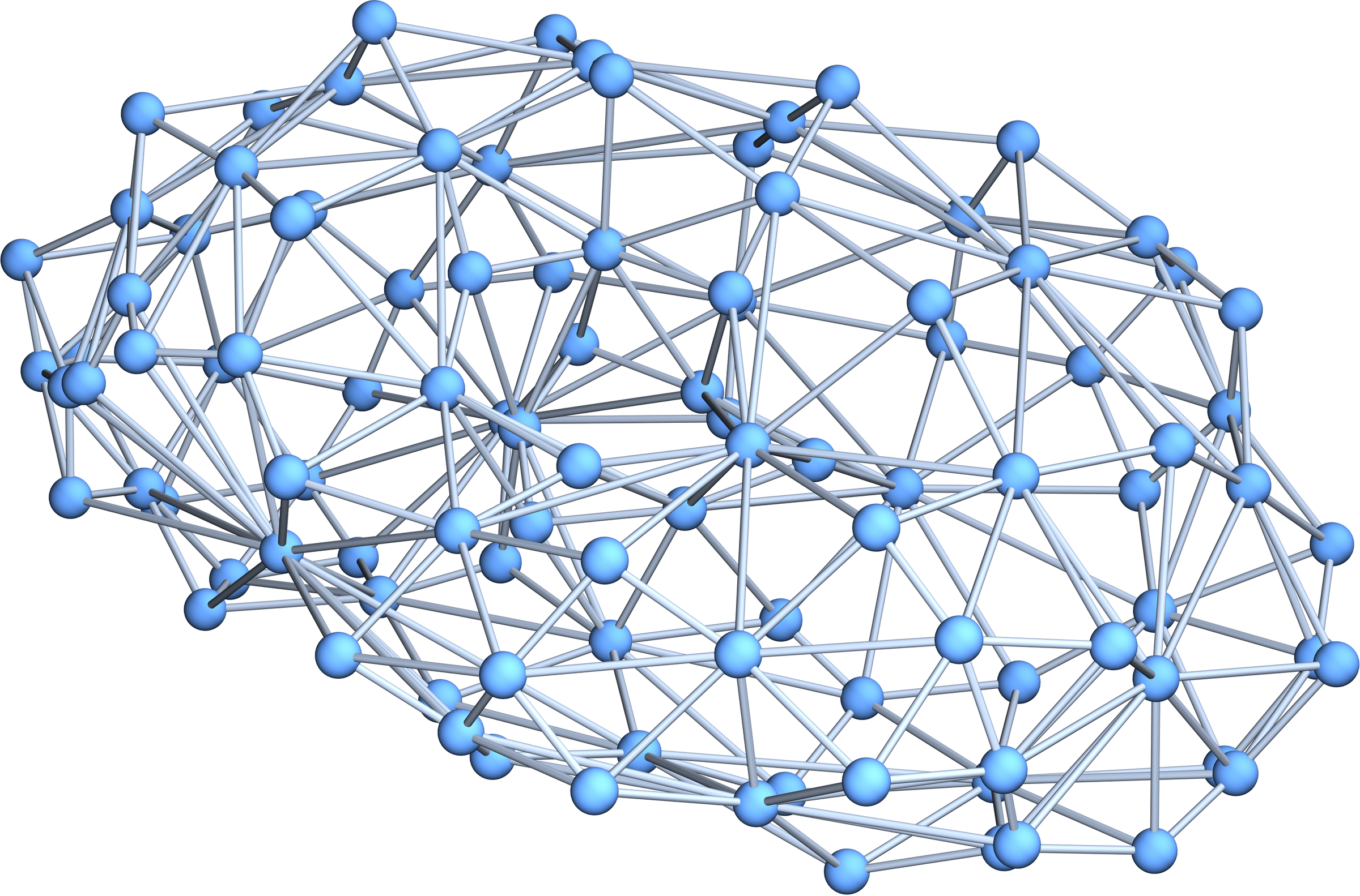
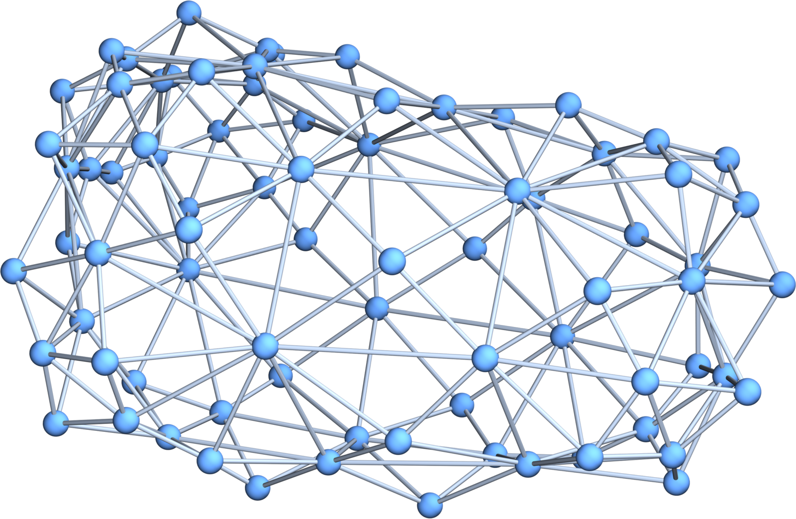
The first surface of co-dimension 2 in the 4-manifold is a 2-torus. The second is a sphere. The first is {f=0,g=0}, the second is {g=0,f=0}. The code above generates random cases. For the picture, I used the following functions f,g leading to the functions called fg,gf from the 4-manifold to 
(* For the picture, I had the following functions *)
P={{3},{4},{1},{2},{3,4},{3,1},{3,2},{4,1},{4,2},{3,4,1},{3,4,2}};
f={1->-0.25,2->-0.05,3->0.35,4->0.25,5->0.16,6->-0.04,7->0.30,8->0.07,9->-0.39,10->-0.29,11->-0.15};
g={1->0.30,2->0.01,3->-0.14,4->-0.14,5->-0.27,6->0.15,7->-0.002,8->0.01,9->-0.29,10->-0.13,11->-0.10};
fg={1->2,2->2,3->3,4->3,5->3,6->2,7->3,8->4,9->1,10->1,11->1};
gf={1->3,2->3,3->2,4->2,5->2,6->3,7->2,8->4,9->1,10->1,11->1};
Hfg=AbstractSurface[G,fg,FF]; Hgf=AbstractSurface[G,gf,FF]; {Betti[Hfg],Betti[Hgf]}
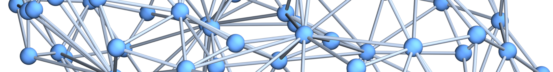
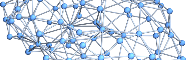
{GraphPlot3D[ToGraph[Hfg]],GraphPlot3D[ToGraph[Hfg]]}