Graph Complements of Cyclic Graphs

Here is some work done over the winter break. PDF , ArXiv and some slides as well as Mathematica code. Just to get to the point, there are interesting new patterns which emerged when studying complements of cyclic graphs. First of all, these graphs are all homotopic to spheres or wedge sums of spheres. Then they have unit spheres which exhibit a universal graph limit universality in that the curvature converges to a 6-periodic attractor. Also the Brouwer-Lefschetz fixed point theory has a 12-periodic feature. These are 2 or 4 periodic features when climbing the dimension ladder using suspensions. The subject is not only interesting in graph theory but also relates to classical topics like differential geometry or algebraic topology. What is nice about this subject is that it combines one of the simplest things imaginable, cyclic graphs (polygons and polygrams) with some of the most exciting topics in mathematics like Gauss-Bonnet, Lefschetz fixed point theory, cohomology, index theorems, combinatorics or universal features.

Bicycle wheels

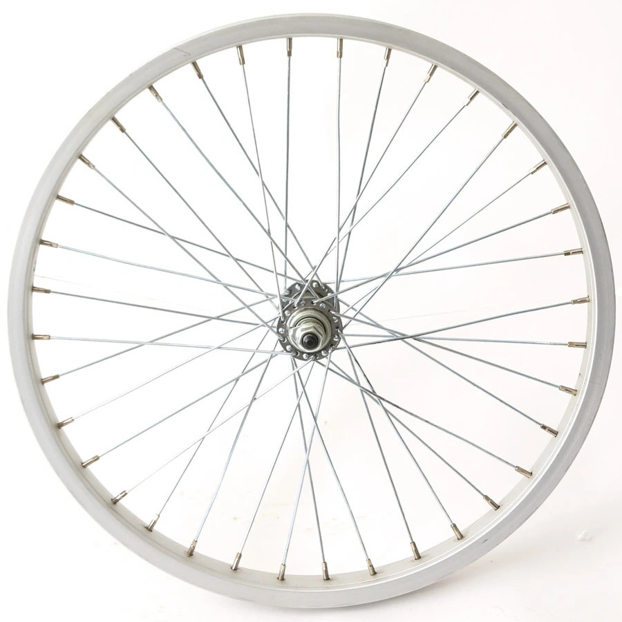
My grandfather Sigbert Bader was not only a sports fanatic, he also ran his own bicycle sell- and repair shop in Neuhausen near the rheinfalls. When we visited, for example to our bikes repaired or wanting a new bike, we would usually work there also for an afternoon, like building bicycle wheels from scratch using basic ingredients like center, rim and spikes. One had to weave in the spikes in a periodic manner and then tune each individual spike so that the wheel is round. It is not so easy. There was a precision tool which allowed to fine tune the tension of each spike. Performing such a mundane task not only leads to an appreciation of what a marvel we have with the concept of a bicycle wheel (it is not as complicated as tensegrity type models) but there is an interplay and equilibrium between forces which makes a wheel stable and robust, also allowing the bike to work in rather uneven environments, like on unpaved streets. And it is good to know how to tune or fix a wheel which is not quite round by adjusting the tension of the individual spikes. This can be done in a clever way without having to remove the tire. But a bicycle wheel spike also has a lot to do with mathematics. It has symmetry, it is a discretization of a concept of a disk with circular boundary. In graph theory, it is related to wheel graphs. In any way, the topic relates to some project I was working on during the winter weeks.

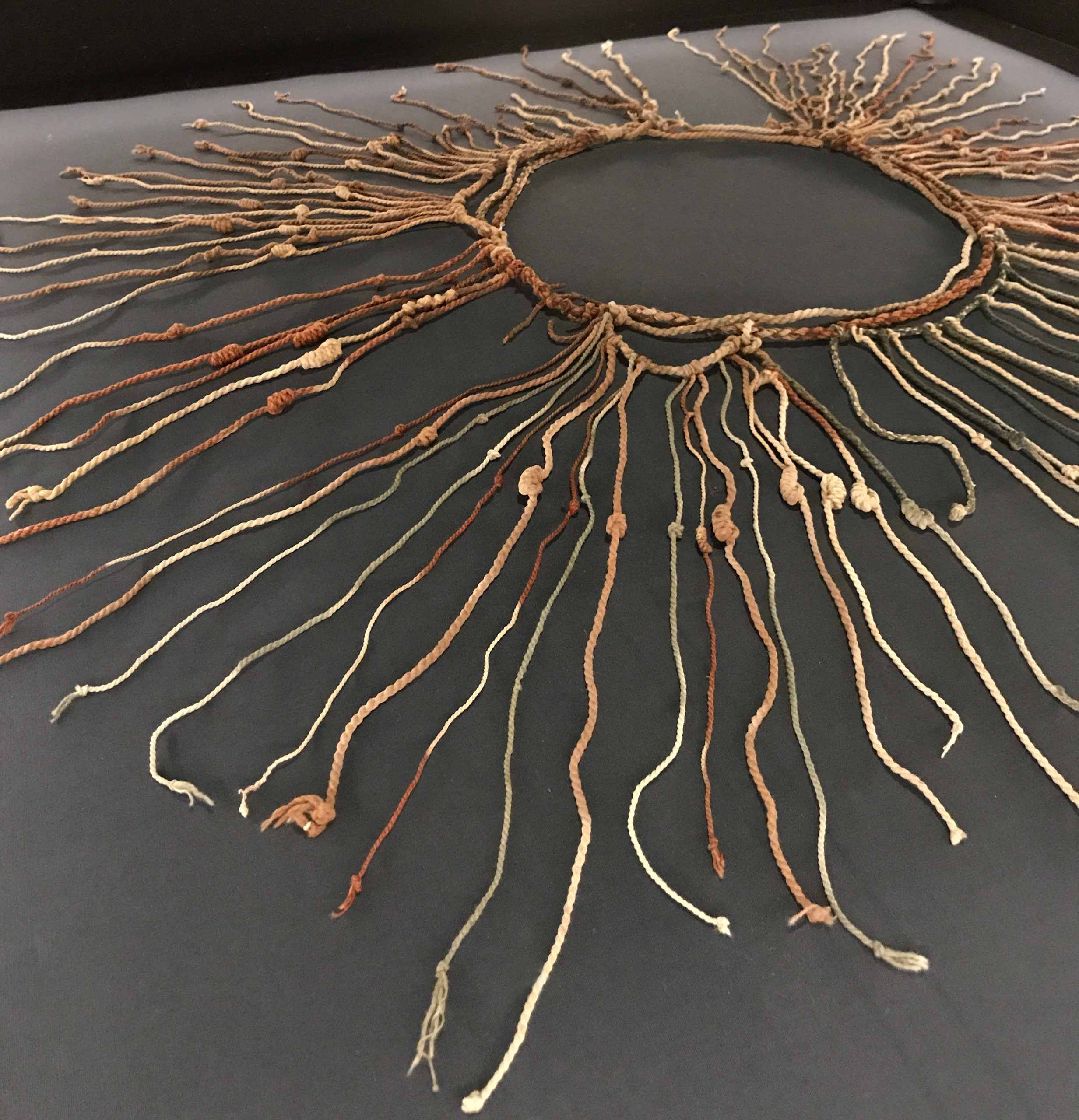
A finite simple graph G=(V,E) is a collection V of nodes and a set E of connections between nodes. The word “simple” means that there are no self loops and no multiple connections allowed. A bicycle wheel is a graph. One can see it as a disjoint union of two cyclic graphs in which some of the nodes on one circle are connected to the nodes on the other circle. Graphs are very intuitive and can be understood already early on. The subject is much more accessible than say calculus. A small kid can read a subway map or a family tree or a directory file system in a computer. The homotopy we refer to is a process which a kid can understand too while the continuum (completely analogue process developed in the 20th century,mostly by mathematicians at MIT) needs at least some training in calculus, due to the appearance of continuity. Even reading letters can be seen as identifying graphs as every letter can be seen as a one-dimensional graph, some being trees like the letter Y, some having loops like the letter B. It might come a bit to a surprise, even for professional mathematicians, that graphs are actually quite powerful. I worked over the last dozen years more and more on graph theory myself and I’m still amazed how much rather serious mathematics actually can be done within graph theory. Somehow it is not surprising, because category theory, is essentially graph theory. The objects of a category are the nodes and the morphisms are connections between these objects. There is something innocent in the concept of finite simple graphs but it actually is quite universal. Similarly as set theory can be used to build up all of mathematics or a relational databases can be used to build up complex information containers, one can also use graphs as a fundamental frame work. As mentioned this can manifest in the language of category theory, in the case of data bases by graph data base. The later is actually quite an old concept too as the Khipu concept shows (I had been in 2018 to get acquainted more with that fascinating topic because I had been on a thesis committee on the subject).

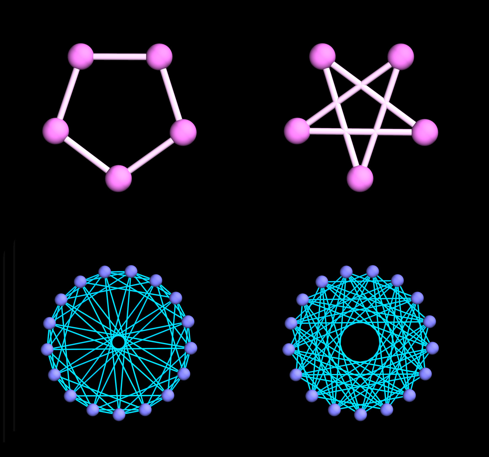
Polygons

oeGiven a finite simple graph G=(V,E) one can look at the graph complement , where is the complement of E in the set of all connections between different nodes. The graph complement of a complete graph with n nodes is the graph with n nodes and no connections. The graph complement of the cyclic graph with 5 nodes is the cyclic graph with 5 nodes again. Taking graph complements is an involution on the class of finite simple graphs and some of the graphs are self-dual, like the pentagon. This might be one reason why pentagons are associated so much with magic, witchcraft or military power. Hexagons, heptagons and octagons are associated to various religions: the hexagon appears in the star of David, the tree of life in the Kabbalah, the heptagon appears in Christianity as a symbol for the 7 days of creation. The octagon is an Islamic symbol of overlapping squares. It is known as the Rub El Hizb or Islamic star. The nonagon finally appears in the Baha’i faith. Related to polygons or cyclic graphs are polygrams, which can be obtained by rearranging the edges in a periodic manner. Like polygons, polygrams are Cayley graphs. The cultural and religious and spiritual fascination with polygons is appalling. It illustrates that symbols and especially symmetry are important, as they are intelligible and visually appealing. There are entire franchises of books and movies which deal with the fascination, in particular the Dan Brown stories, like Angels and Demons. There is an entire aspect of geometry called sacred geometry which had historically been a driving force for studying geometry. In modern times this motivation of course has long faded but symmetry remains to have appeal. Also non-kids can get mesmerized by a caleidoscope. Also some naturally occurring networks like orbital networks often show symmetry.

Circulant graphs

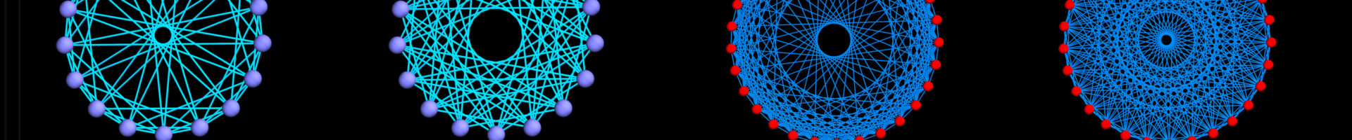
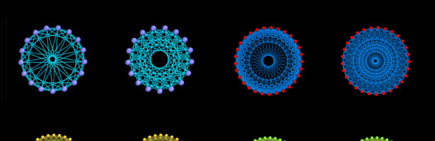
All these graphs are examples of circulant graphs. For a mathematician, they are Cayley graphs defined by a set of relations generating the Abelian cyclic group . The most obvious generator produces the cyclic graphs, but one can also use other generators and the connectivity of the corresponding graph can depend on number theoretical issues. Take take the generator for example. It generates two disconnected 4-gons because 2 is divisible by 8. Also the star of David can be seen as an overlap of two disconnected triangles. For such circulant graphs, the graph complement is again a circulant graph but we just replace the set of generators by the complement in the set of all possible generators. In other words, we take the generators . Graph theory can be studied on various levels. One can look at combinatorial problems like counting subgraphs, one can look at topological features like connectivity, dimension or simply connectivity, one can also look at the topology of geometric realizations of a simplicial complex defined by the graph. The Whitney complex is the most natural complex on a graph: it is generated by the complete subgraphs. The geometric realizations can have very complex homotopy and cohomology types. I started this subject by computing cohomology groups. When talking about geometric realizations is only done in order to motivate, it is never needed. [ Indeed, if tomorrow, somebody would find an inconsistency in ZFC (which is possible and by Goedel completely futile to be ruled out by proof), then this is core finite mathematics which would survive also such a cataclysmic event and remain true if we should decide to get rid of the concept of “infinity”. I myself got more and more convinced over the last decade that we actually do not need the infinity axiom at all. All we humans do and ever will be able to do is to access and process finite data using finite computing devices like our brains or computers. Infinity is an idealization which helps to build theories but these theories (like differential geometry) can be substituted by finite objects too. The developments of computer graphics shows this. Of course, 99 percent of mathematics relies on the continuum and has not been translated in a satisfactory way to the discrete. Not that there are any doubts that it can not, as any numerical computer simulation is process on finite sets, but that the language can be adapted in an elegant way. A prototype how this can be done is radically elementary probability theory by Ed Nelson or discrete integral geometry by Klain and Rota or Regge calculus in general relativity. ]

Cohomology groups

Cohomology theory is usually presented in a way which only can be accessed after having studied at least 2 semesters of mathematics. Especially axiomatic approaches or techniques that develop diagram chasing techniques need time to be digested. They usually seem to be learned by intimidation or by referring to authority. I myself learned it as a junior in college have difficulties with most algebraic topology books and “dig” the older texts like Alexandrov’s combinatorial topology. The simplest approach to cohomology is definitely the one by William Hodge who was eight years old when Poincare died but still can be considered to be a modern mathematicians. The approach only requires to know what a matrix and its kernel is and so can be absorbed easily after having seen a few weeks of linear algebra. Define a concrete matrix d, the incidence matrix first, then define the Dirac matrix D=d+d* and finally the matrix H=D². This is a partitioned matrix for which one can compute the nullity of the k’th block. This is the k’th Betti number. I have used Hodge Laplacian eigenvalue computations examples for years (sometimes hidden) in basic linear algebra courses and know that also non-mathematician teenagers can get this. On the other hand, reading algebraic topology books needs some mathematical maturity. So, here is how we can compute the cohomology groups of the graph G_n which is the graph complement of the cyclic graph C_n. The matrix is a matrix if there are n complete subgraphs in the graph. For any pair (x,y) of subgraphs, define the matrix entry which is either 1 or -1 depending on whether has a compatible induced orientation on y or not. Otherwise if x is not a subset of y, define d(x,y)=0. The matrix is the Dirac operator, the matrix is the Hodge Laplacian. The matrix d is the exterior derivative which is known as gradient, curl or divergence in multi-variable calculus in . It satisfies which we known in calculus as . The Dirac matrix is something which mathematicians like Betti, Poincaré, Noether or Hopf could have come up with but which they missed. (One explanation is the Dirac operator was appreciated only much later, in particular with work of Atiyah, a student of Hodge. One can see in the literature several different implementations of the Dirac operator in the discrete, often trying to copy the Clifford algebra construction from the continuum, which is completely unnecessary in the discrete). The matrix depends on a given order of the subsets but this order is as arbitrary as if we use an xy coordinate system or yx coordinate system in linear algebra, it is just a choice of basis. The spectrum of D is symmetric with respect to 0. (The point of Dirac to introduce a square root of the Laplacian was to get compatibility with special relativity. It lead to anti-particles.) The matrix H does not depend on the choice of orientation for the simplices. It has by definition non-negative eigenvalues only. The 6 lines of code have appeared on this blog already. It is the same code I have always used and for example also used to discover (the rather obvious fact) that McKean-Singer symmetry also holds in the discrete. See also this Wolfram community blog.

ClearAll["Global`*"];
ComputeCohomologyOfCycleGraphComplement[M_]:=Module[{},
Generate[A_]:=Delete[Union[Sort[Flatten[Map[Subsets,A],1]]],1];
check[x_]:=Module[{t=True,m=Length[x]},
  Do[t=And[t,Less[1,Abs[x[[k]]-x[[l]]],M-1]],{k,m},{l,k+1,m}];t];
R=Generate[{Range[M]}]; G={};
Do[x=R[[k]];If[check[x],G=Append[G,x]],{k,Length[R]}];
n=Length[G]; Dim=Map[Length,G]-1;f=Delete[BinCounts[Dim],1];
Omega[x_]:=-(-1)^Length[x]; EulerChi=Total[Map[Omega,G]];
Orient[a_,b_]:=Module[{z,c,k=Length[a],l=Length[b]},
  If[SubsetQ[a,b] && (k==l+1),z=Complement[a,b][[1]];
  c=Prepend[b,z]; Signature[a]*Signature[c],0]];
d=Table[Orient[G[[i]],G[[j]]],{i,n},{j,n}];Dirac=d+Transpose[d];
H=Dirac.Dirac; f=Prepend[f,0]; m=Length[f]-1;
U=Table[v=f[[k+1]];Table[u=Sum[f[[l]],{l,k}];H[[u+i,u+j]],{i,v},{j,v}],{k,m}];
Cohomology = Map[NullSpace,U]; 
Betti=Map[Length,Cohomology]]

ComputeCohomologyOfCycleGraphComplement[11]

Export["hodge.gif",
Animate[MatrixPlot[Re[MatrixExp[1.0tI H]]], {t, 0, 2, 0.1}], "GIF"];

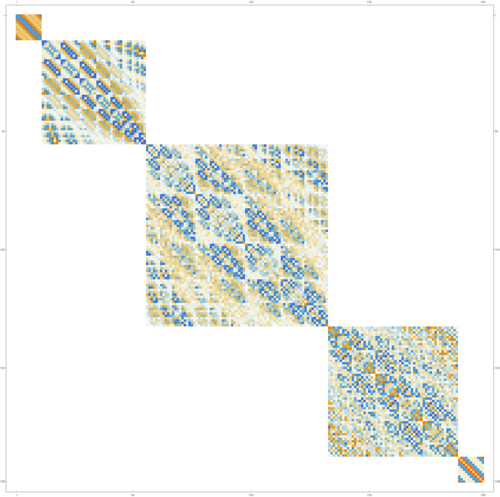
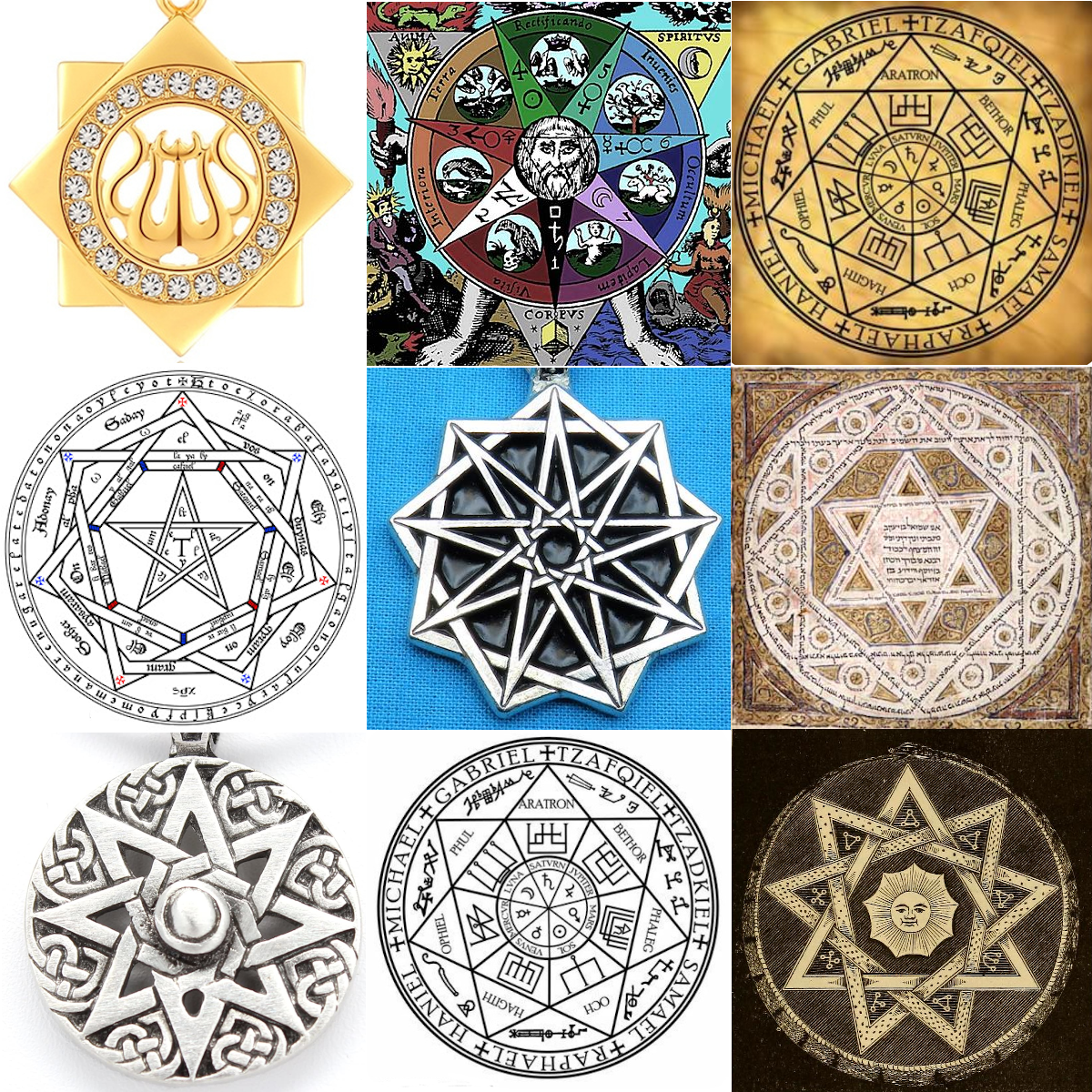
We get the result (1,0,0,1,0) which means the Betti vector is (1,0,0,1). It is the Betti vector a 3-sphere. You can experiment yourself and see that for M=12, we get (1,0,0,2,0) which indicates that the topological space is homotopic to a wedge sum of two 3-spheres. This is indeed the case. Doing such computations was for me the starting point of this research done over this winter month. What is fascinating, is that one of the simplest topics in mathematics, the concept of polygons which is understood already for smaller kids and present in primitive religious symbols relates to rather modern mathematics like stable homotopy theory as we can look what happens to these spaces when we disregard the process of suspension which is here just appears as the third power of the operation of increasing the size of the polygon by 1. By the way, the code above also plotted the matrix M. We actually plotted the real part of the Schrödinger unitary evolution matrix cos(H) =Re(exp(i H) ) in order to see the block structure better. There is rather serious mathematics involved when dealing with such objects in the continuum. It is related to Atiyah-Singer stuff, related to interesting quantum mechanics and geometry. So here is the matrix cos(H). Afterwards, we show the GIF animation which shows the Schrödinger evolution. We have computed with 12 lines of computer code (from scratch without any libraries) a movie of the Schrödinger wave evolution of a quantum wave evolving on a 3-dimensional sphere modeled by a simplicial complex with 198 simplices and the computation is done on all differentrial forms in parallel! Dodge that !