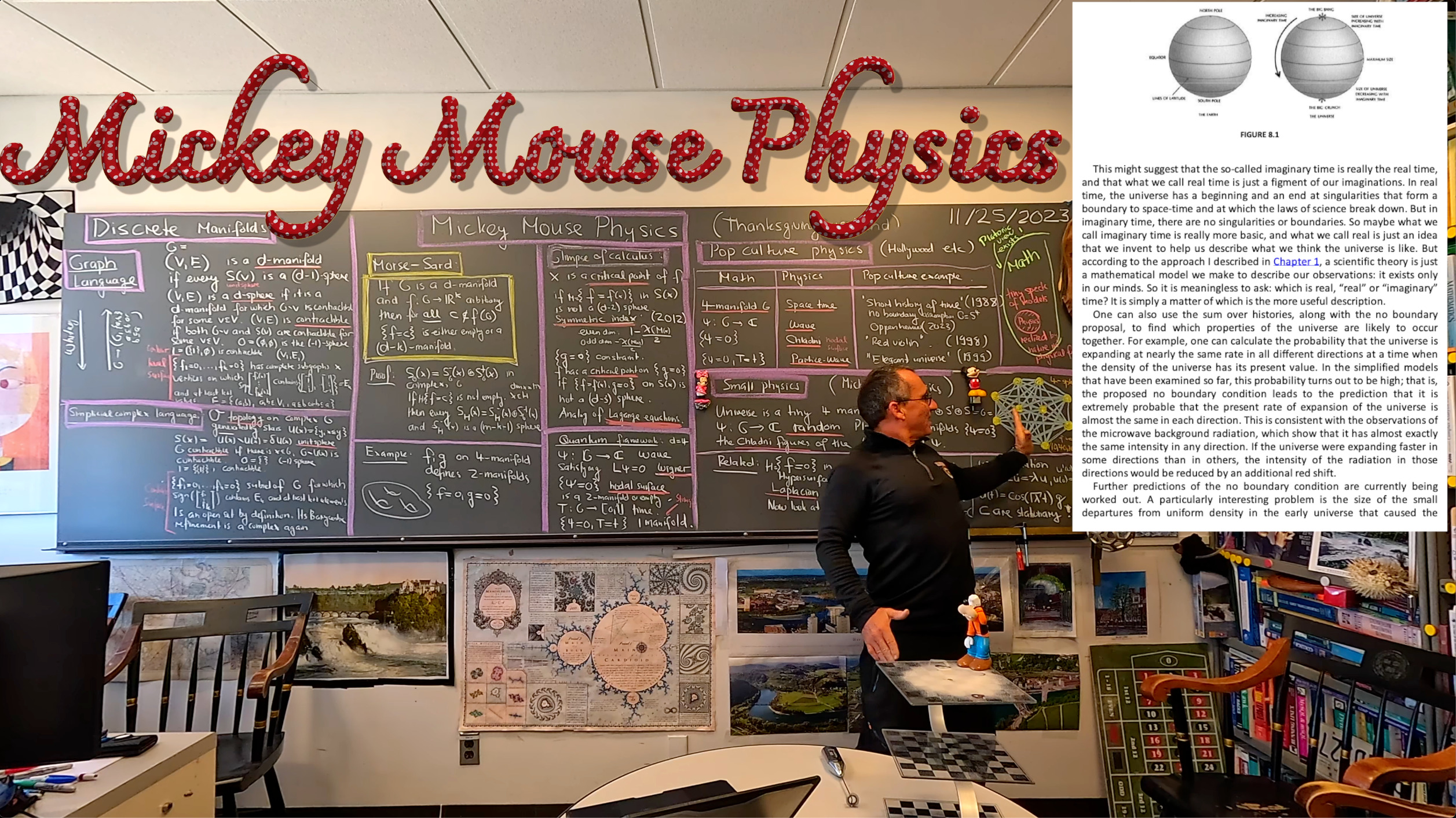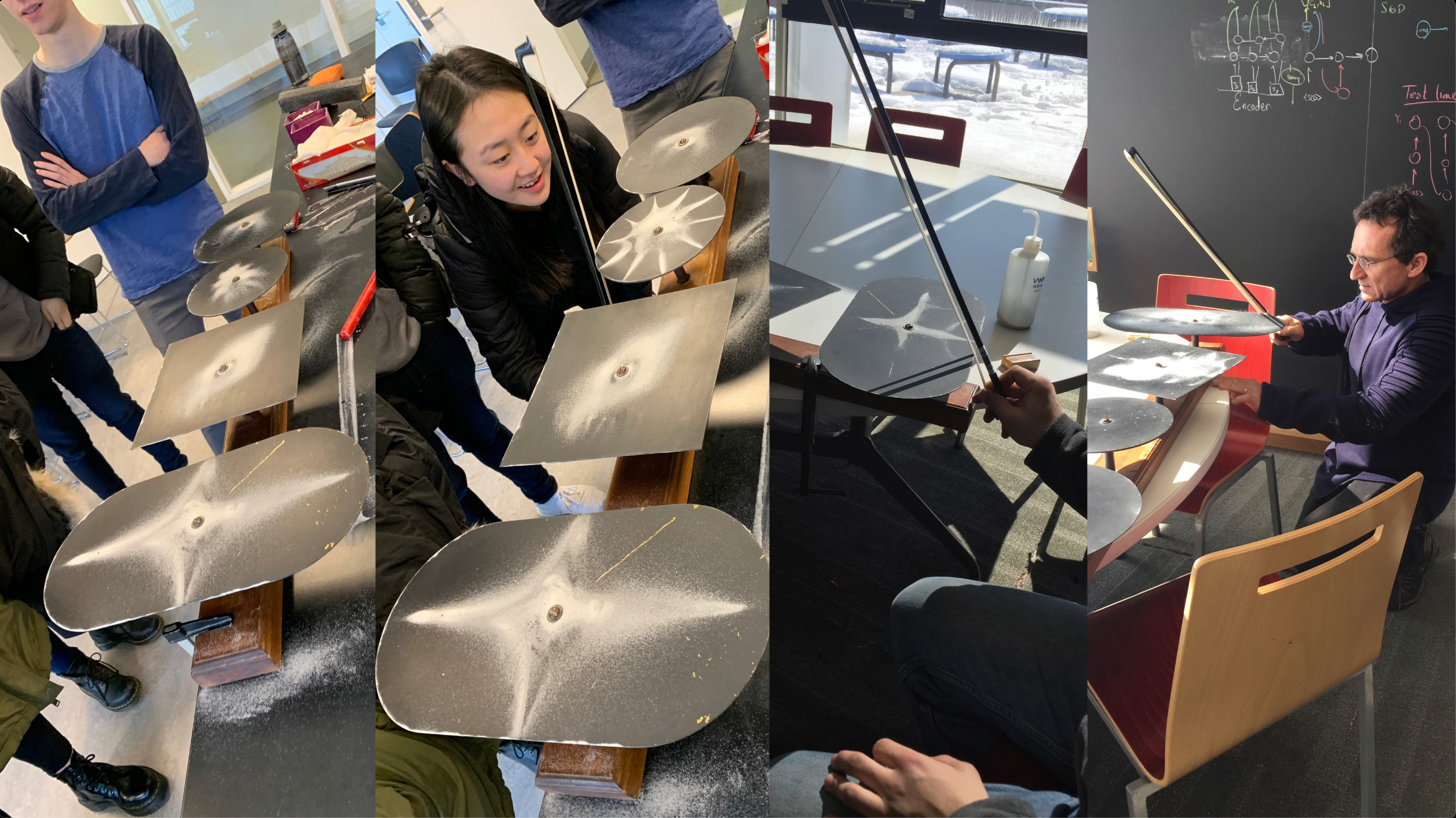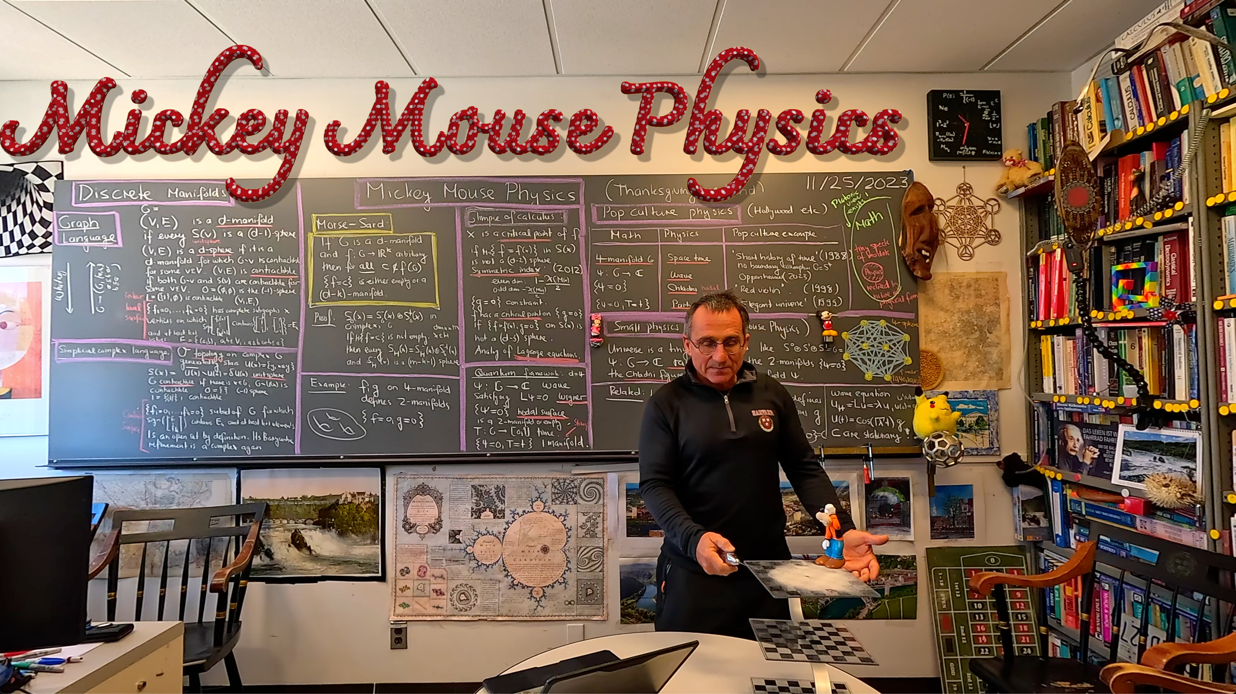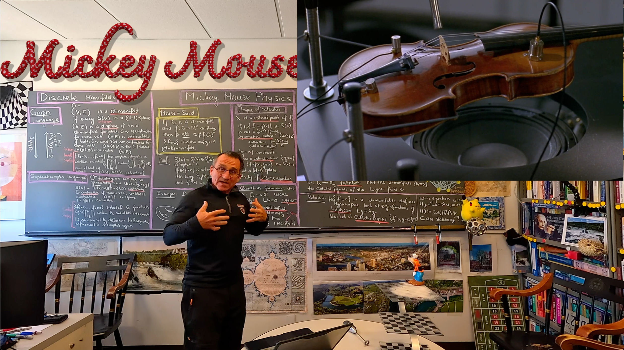
One of the nice things in mathematics is that one can play with models which do not necessarily have to do directly with the real world, whatever the later means. We can look at abstract objects, like finite simple groups, number theory in some number field or topology in 1001 dimensions. The physical theories make up only a tiny part of the mathematical world (which for most mathematicians exist even without discovery). Mathematicians can tease their physics friends because they only consider a tiny speck in a much larger mathematical universe. And physicists can tease their chemistry friends that their world occupies only a tiny speck in the world of physics. And chemists can tease their biology friends pointing out that their world lives in a tiny speck in the much larger world of chemistry. There is a famous XKCD cartoon about this, with a slightly different order relation “applied part” instead of “contained in”. The later twist by the way, I had used myself (long before XKCD existed!) as a high school student after deciding to study math. It would go like this: “So, you study chemistry? Cool. That’s part of physics. And physics is part of math, which is what I will study. We have something in common”, the point inducing of course in a nasty way (teenagers!) that the common part is not an intersection but an inclusion used in a case where inclusion is quite offensive as it means “limiting”.
There is no lack of offense from the other side of course like seeing math as a “tool” or a “language” or a “frame work” to do “more important stuff”. Or then the arrogance of other departments not only snatching away entire chunks of math into their own (no offense there, that is fair competition) but brutally abducting a computer away from mathematics to computer science (lots of offense here!) or forcing mathematicians to “include messy data” into their courses and diluting the elegance, beauty and poetry of math with entering data into spreadsheets and claiming that this is “data science”. Also pure mathematicians are naturally data scientists: every serious mathematician has to process hundreds of books, thousands of papers, do zillions of thought experiments and evaluate the results, discarding results that do not work in order to come up with new models, new theories and new theorems. Pure mathematicians have since antiquity been under pressure of justifying and defending their work because it might be not applied enough for a general public. It is time that pure mathematicians develop more spine and confidence. Some of the most applied, most profitable and most useful things are based on mathematics: we can see inside the body using tomography, compress data using sophisticated algorithms (both based on Fourier theory), communicate in a secure way using basic results in pure number theory (prime numbers). And this was just the beginning, almost everything we do from finance over computer vision to get into space is based on important principles first discovered in pure mathematics.
The development of the discrete Morse-Sard theorem (even it is Mickey-Mouse stuff) needed years of work, millions of experiments, pursuing many, many wrong paths. Looking at lots and lots of data (maybe not in spread sheet form) but in geometric form. It evolved in stages: first in 2015 for one function but only now, this fall with more functions. It might be a small Mickey mouse thing but it is a deliverable. Since last week, not much has happened. I cleaned up and optimized computer algebra programs to experiment including for example to compute the cohomology of any level surface directly without going to the Barycentric refinement. This technically means computing the cohomology of open sets (a special case of Delta sets as by definition the level surfaces are only open sets and not simplicial complexes. I used in the past compute the cohomology by first writing down the graph of the Delta set but it is much faster to compute the cohomology directly in the Delta set. I always bragged about being able to compute all cohomology groups in one sweep with 5 lines of Mathematica code (without any libraries!) and computing the cohomology of discrete algebraic sets 
On the theoretical side, I realized that (a small matter but elegance is important): we do not need at all the assumption that the functions are colorings. The Morse-Sard theorem works in general: let G be any d-manifold and 
")

")
For example, if 


")

 = {\rm Re}(c)")
 = {\rm Im}(c) \}")
")


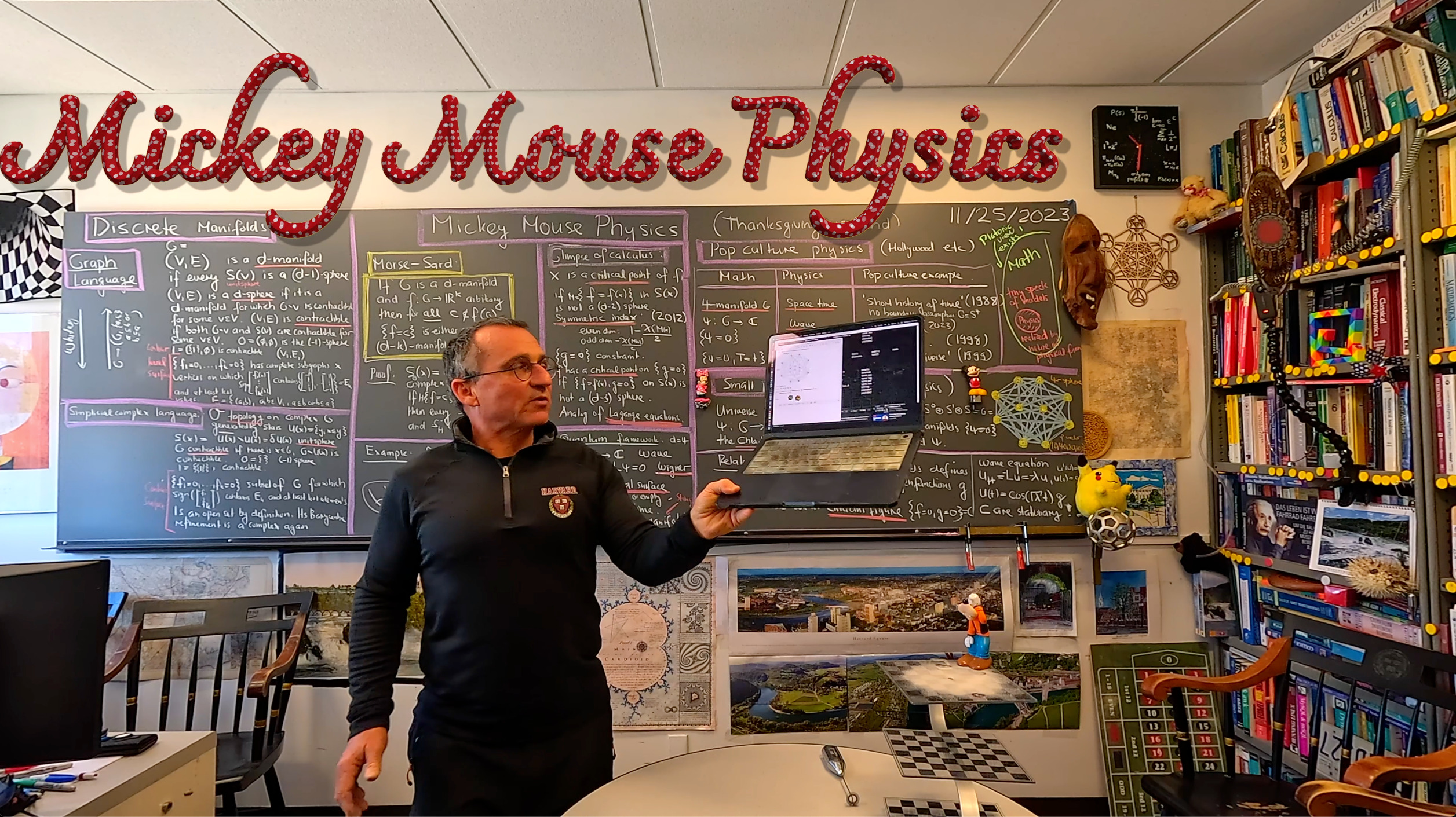
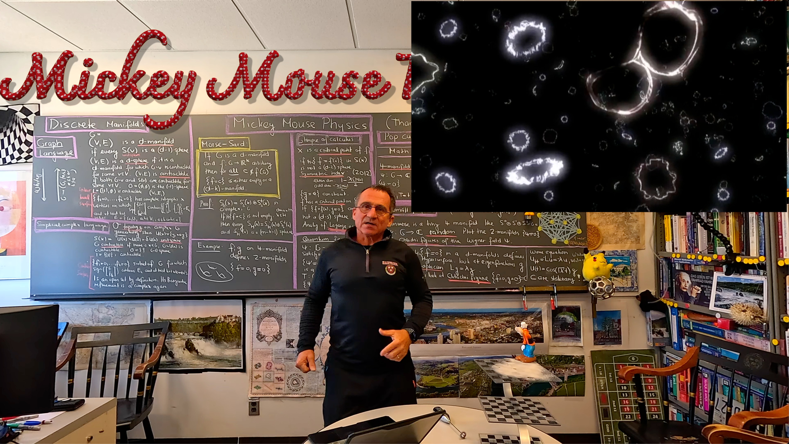
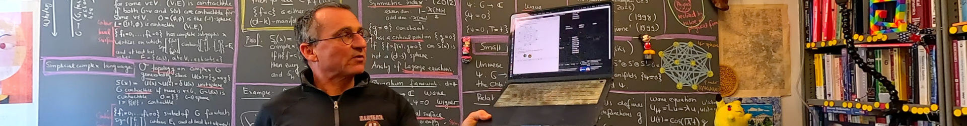
Lets just show an example of a computation done recently. The full code will be released later. But for now, it is a blackbox (52 lines of code so far where much is used just to make the graphics (like taking a graph apart and drawing again the triangles, tubes and spheres rather than taking the default graphics). The following code just search for a higher genus random surface. For the smallest 4 sphere, one sees lots of 2 spheres the largest genus surfaces are tori (genus 0 surfaces) as codimension 1 surfaces. When making the host graph a bit larger, one can increase the genus. It is possible to see genus 2 surfaces already is to take the join of cyclic graphs C5 and C4 and take a suspension of this. The code should be self-explanatory. Whitney is the Whitney functor producing from a graph a simplicial complex. GemPlot is a more sophisticated GraphPlot3D, where also triangles (complete subgraphs of dimension 2) are drawn as polygons. I did not yet figure out how to visualize things nicely if I want to see an evolution of surfaces in the same host graph. Showing it in the small universe (host graph) does not look good yet but we will get there also eventually.
<< code.m;
s = GraphSuspension[GraphJoin[CycleGraph[5], CycleGraph[4]]]; G = Whitney[s]; min = 0;
Do[psi = ComplexRFunction[G]; H = ComplexLevelSurface[G, psi];
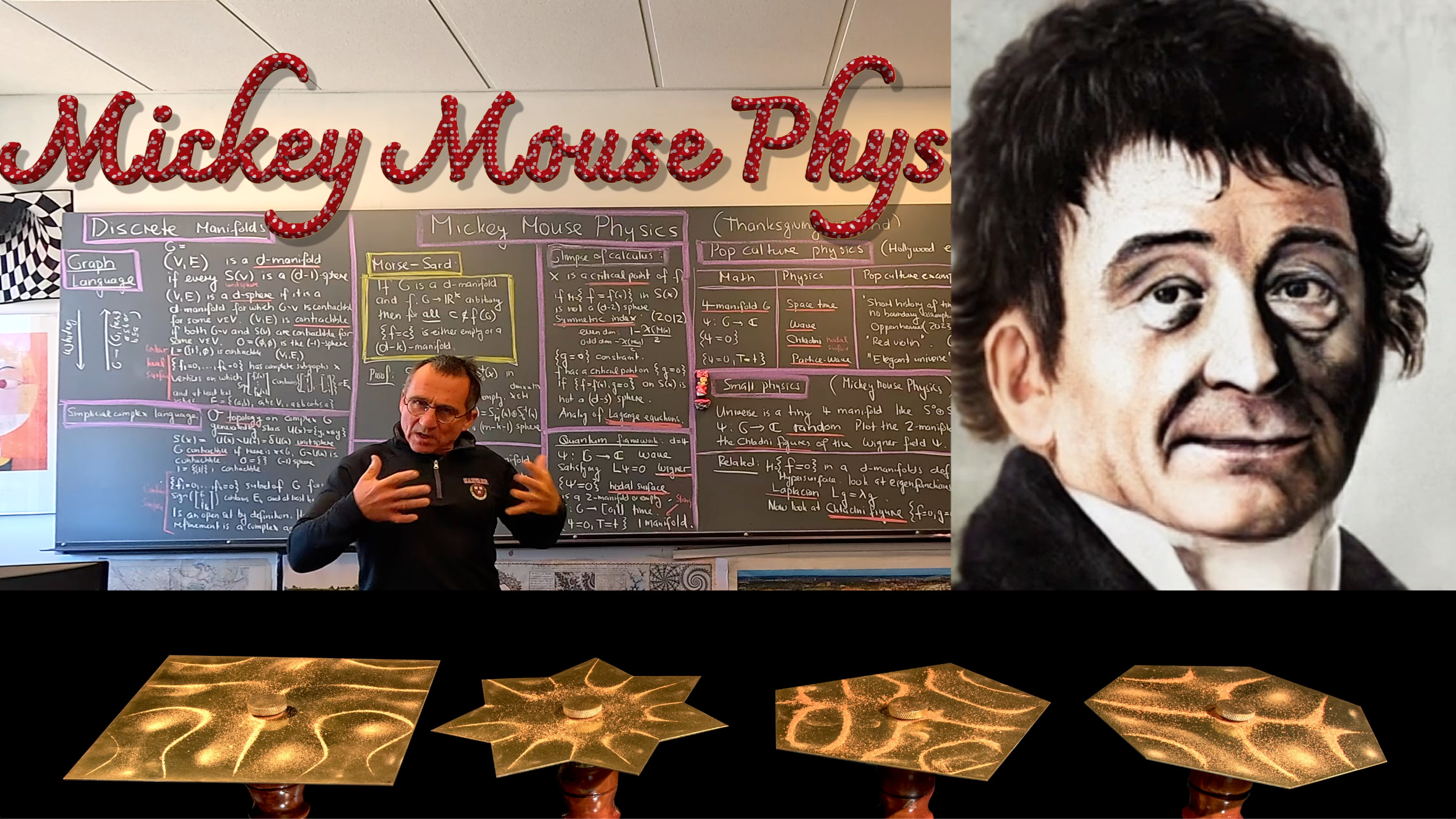
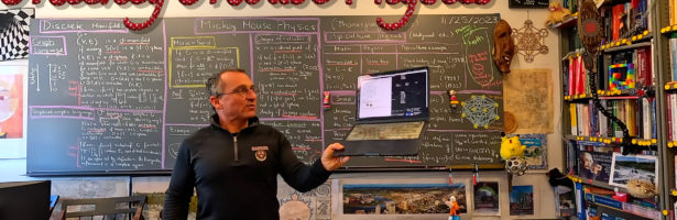
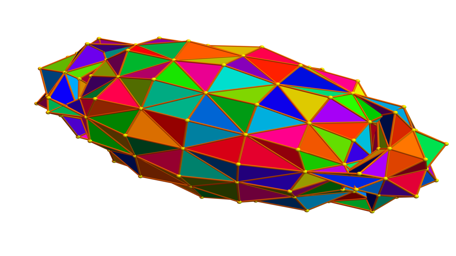
X = EulerChi[H]; If[X < min, min = X; K = H], {5000}]; Print[min]; GemPlot[K]Here is the output. The middle one is a genus 1 surface with Euler characteristic 0 obtained with the above code. Most of the level surfaces are usually 2-spheres or collections of 2-spheres. The right one is a genus 2 example in a G=P2+C6+C4 sphere. Note that all of these examples are 2-manifolds, meaning that every unit sphere in that surface is a cyclic graph with 4 or more elements and the above code picks an example from 5000 examples with maximal genus. That the surfaces are always 2-manifolds or empty is what the discrete Morse Sard theorem tells. And the theorem works in any dimension with any number of functions. It is actually quite remarkable that without almost any effort, we have generated a relatively small genus 2 surface. I had before that always done it either by doing some gluing or taking a level surface f(x,y,z)=c for a suitable function then discretize this. See this page for an exercise I gave to Math 22a students in 2018. The number of nodes one gets by traditionally gluing 2-tori using level surfaces is much larger. I hope to use the program to generate some interesting 3 or 4 manifolds in the future.
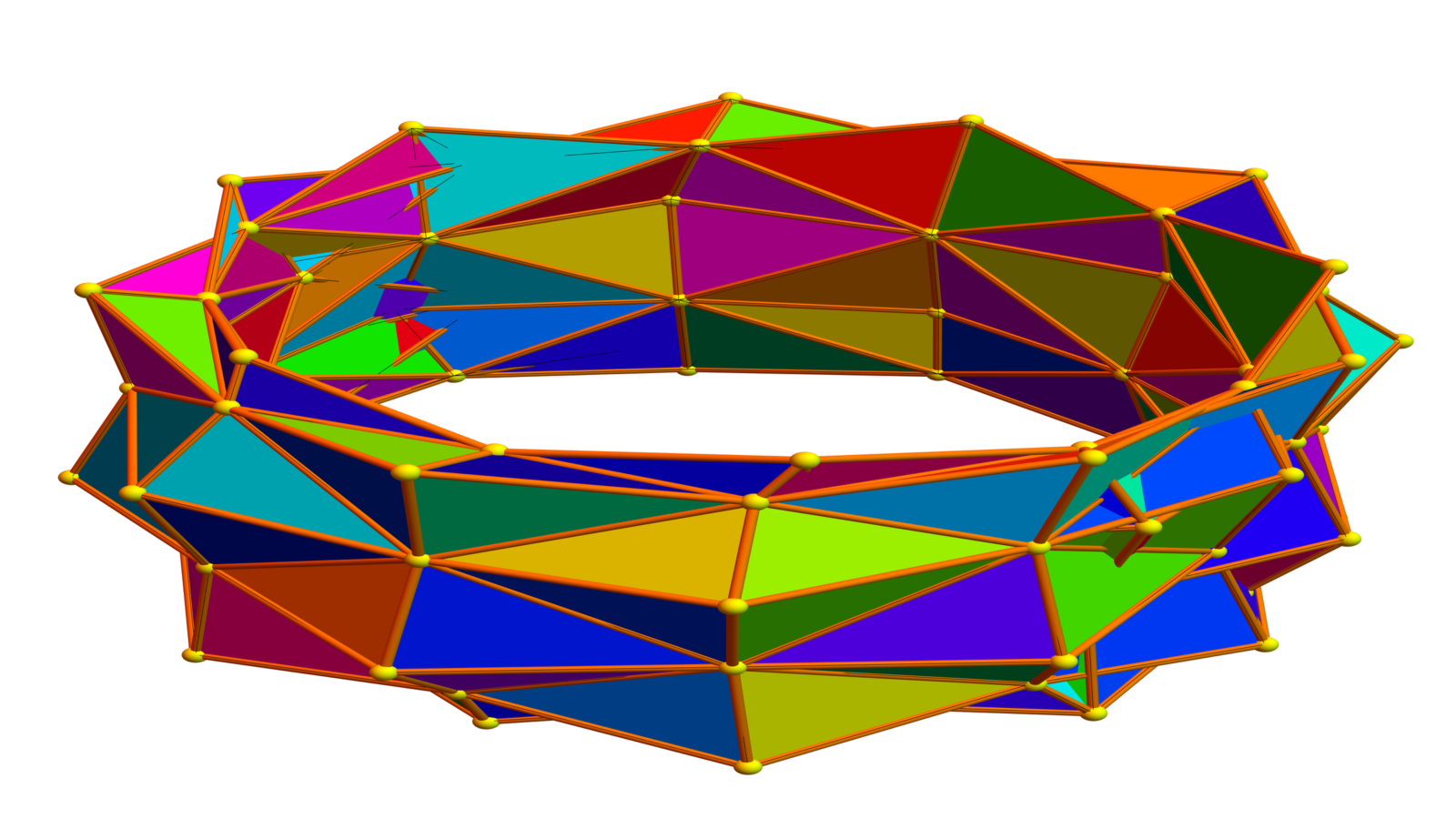
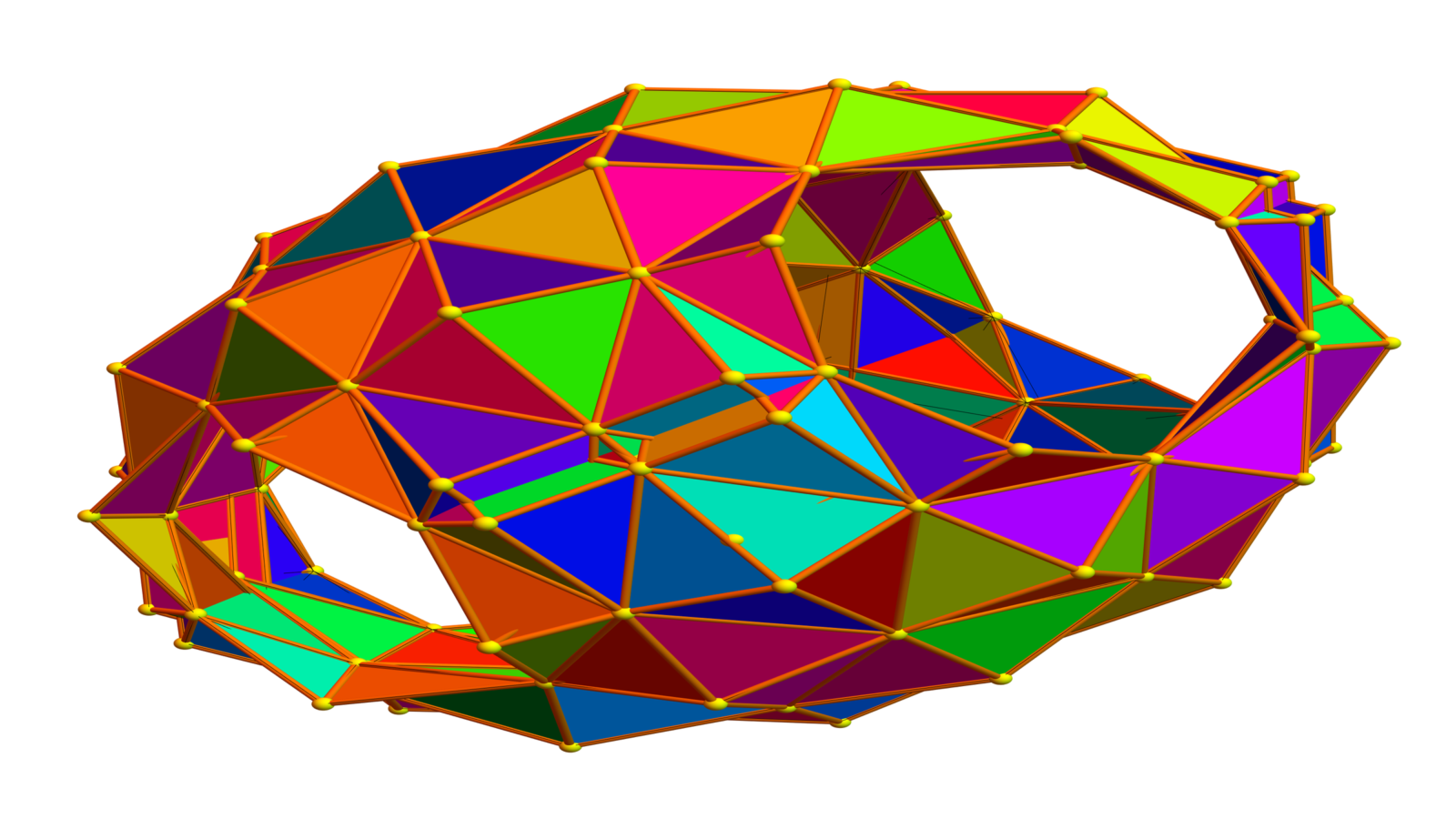
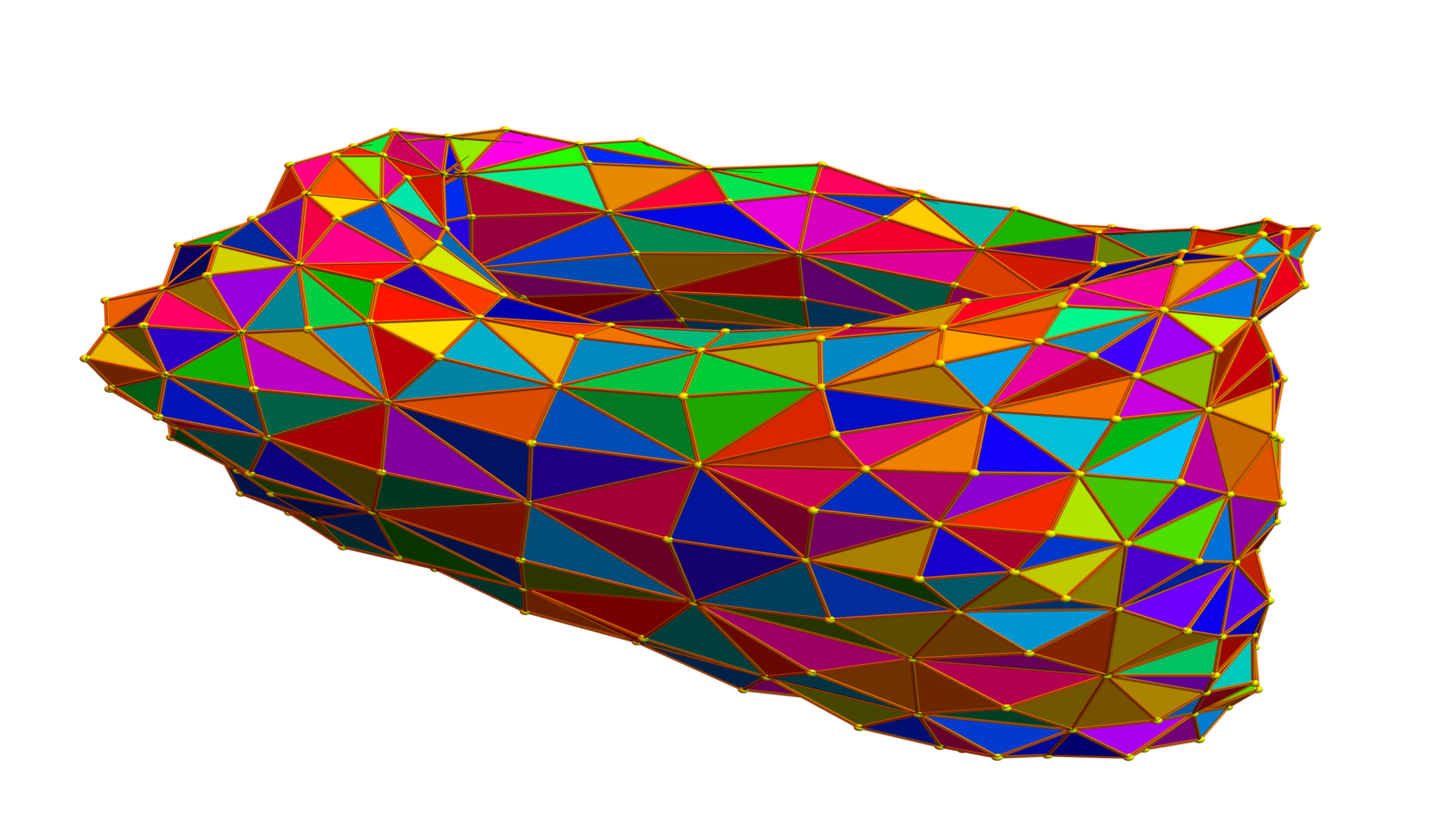
 using a random function. It has 394 sets with f-vector (87,198,109). What we see is the graph with 394 nodes. The simplicial complex of this graph is much larger (the Barycentric refinement of the delta set we actually deal with. The f-vector of the graph is already larger (394, 1050, 654)). It is easy to see that level surfaces in an orientable host graph are orientable. To get non-orientable surfaces like the Klein bottle, one needs to start with a non-orientable 4-manifold. The projective 4 space is the smallest one. The surface above is a 2-manifold with Betti vector (1,3,0). It is obtained by attaching a handle to the Klein bottle. The Klein bottle has Betti vector (1,1,0).
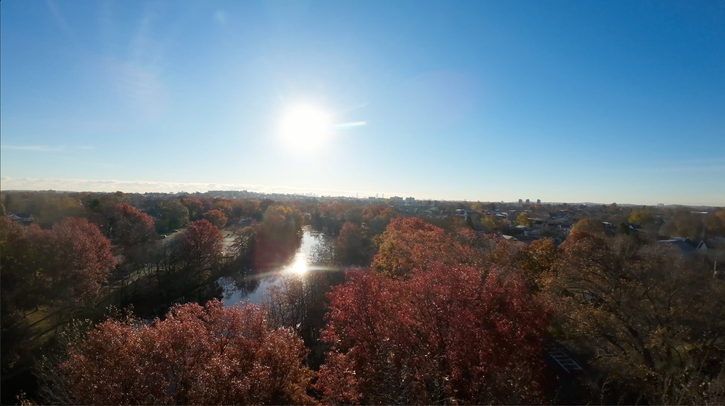
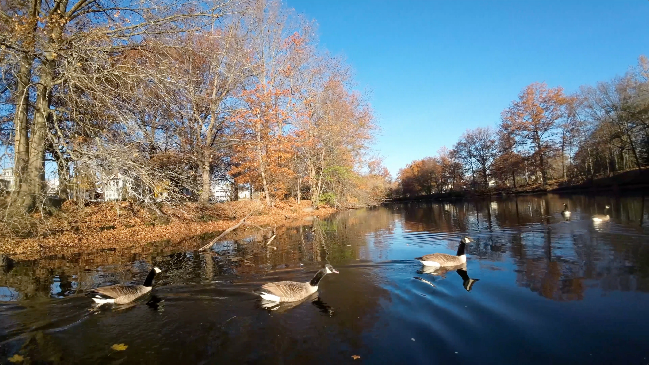
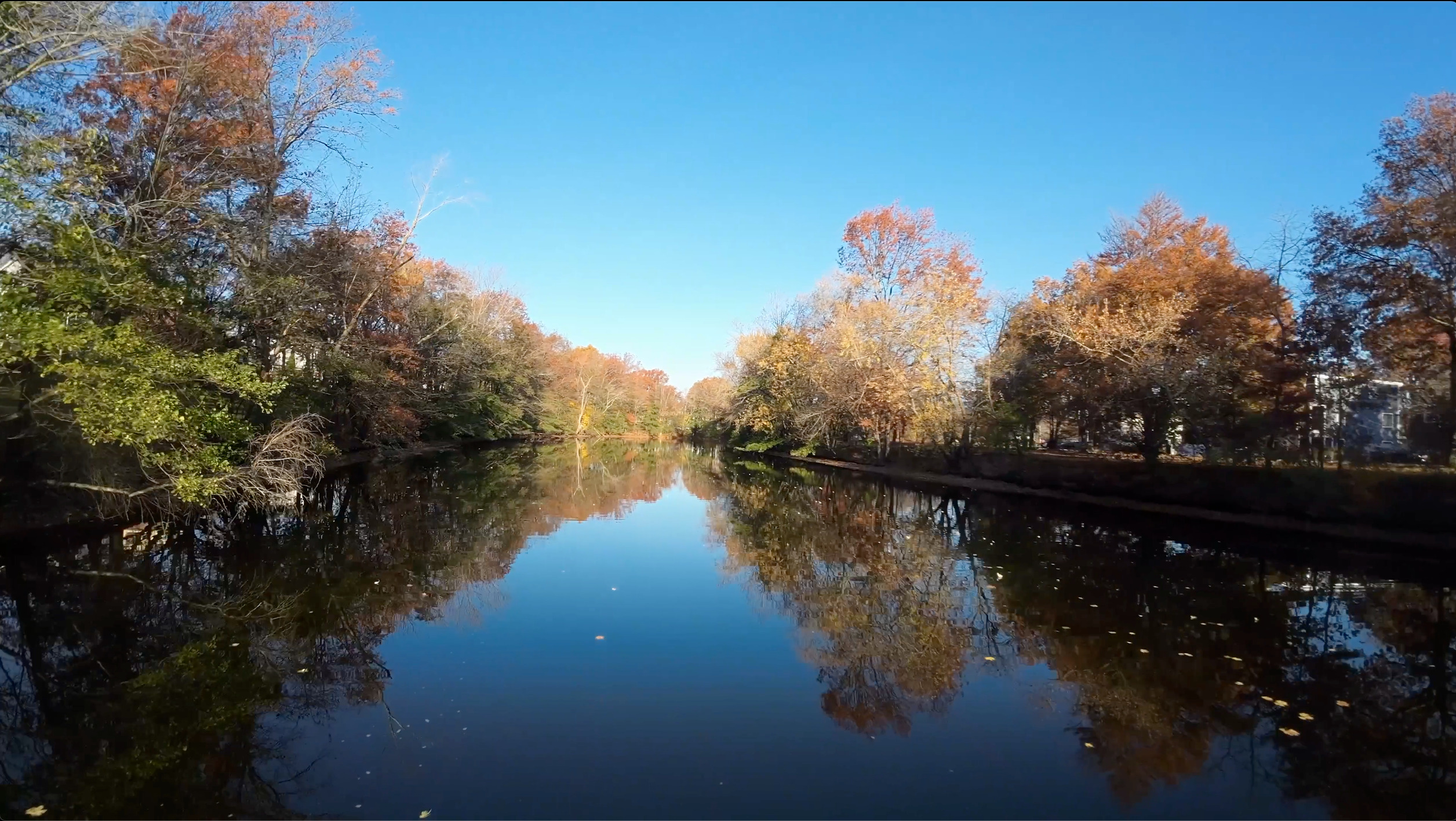
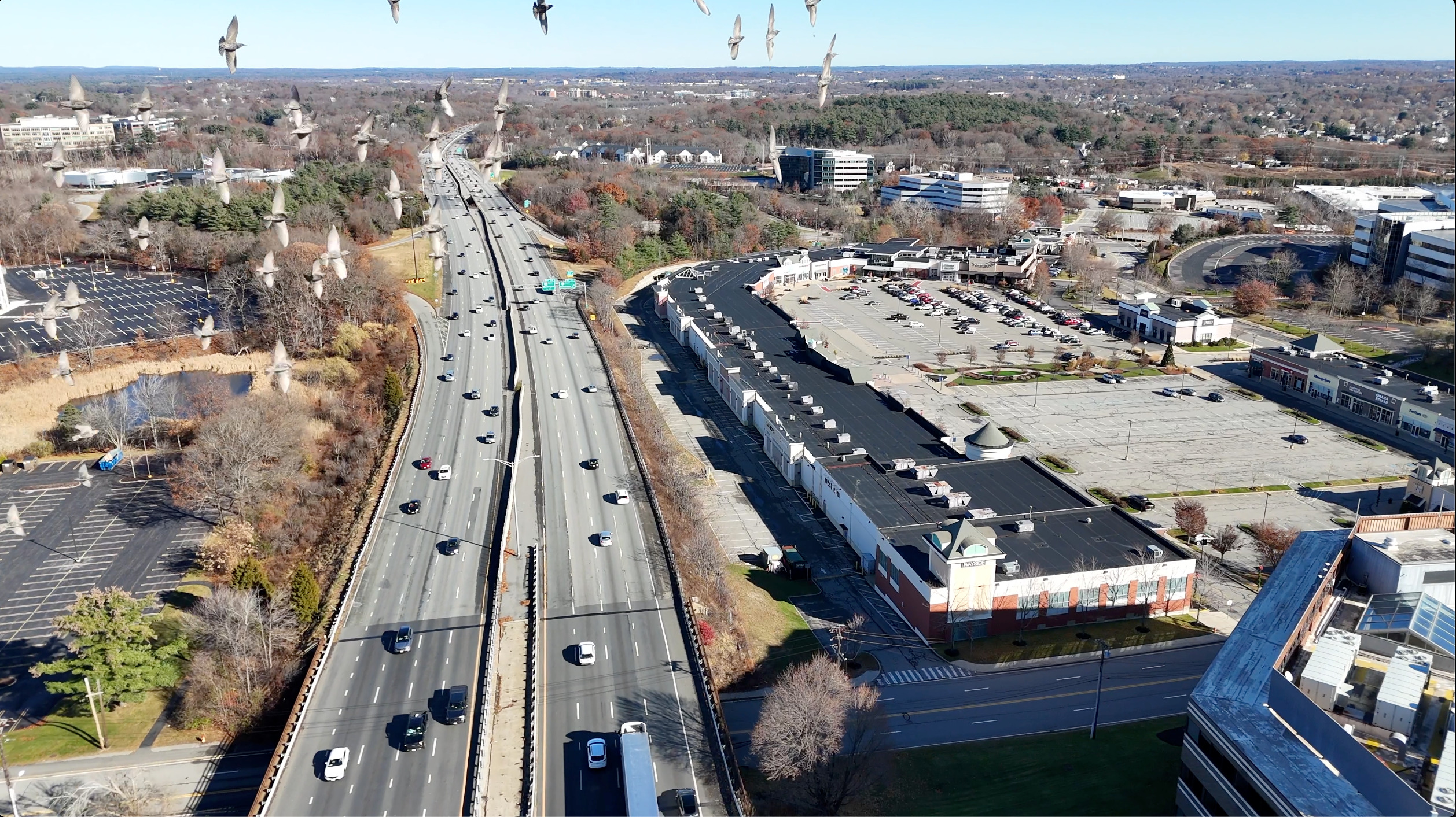
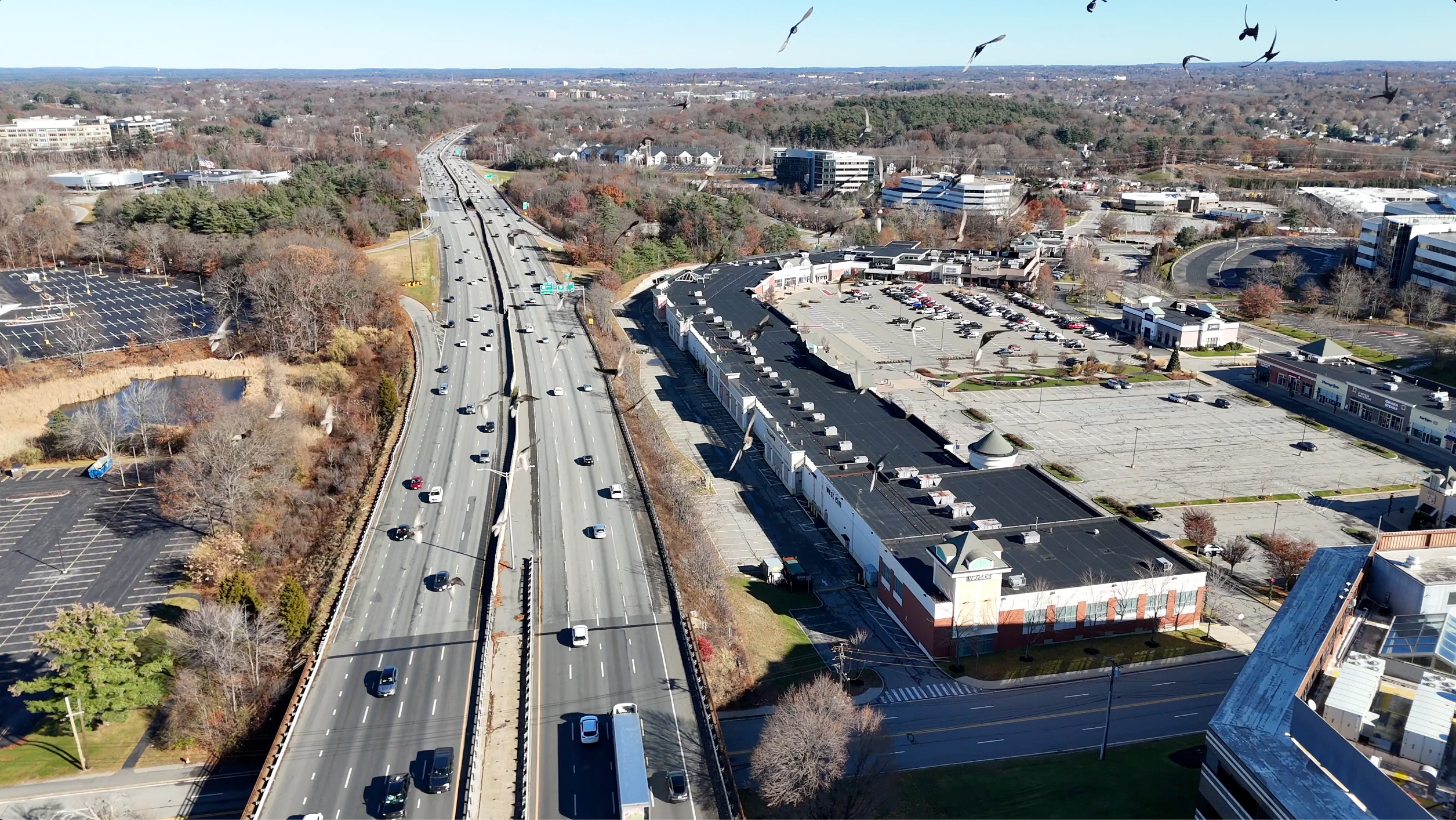
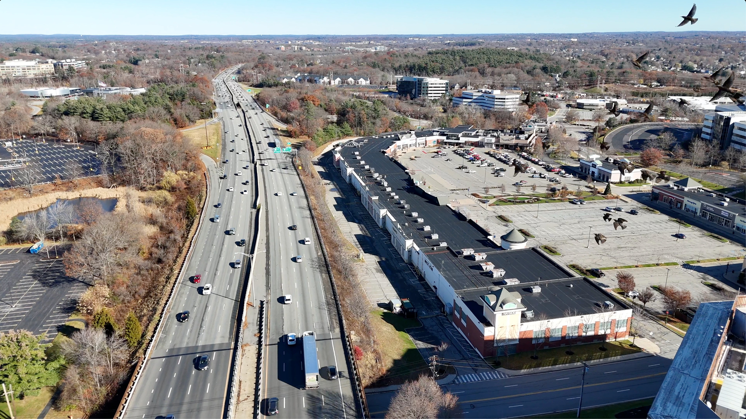
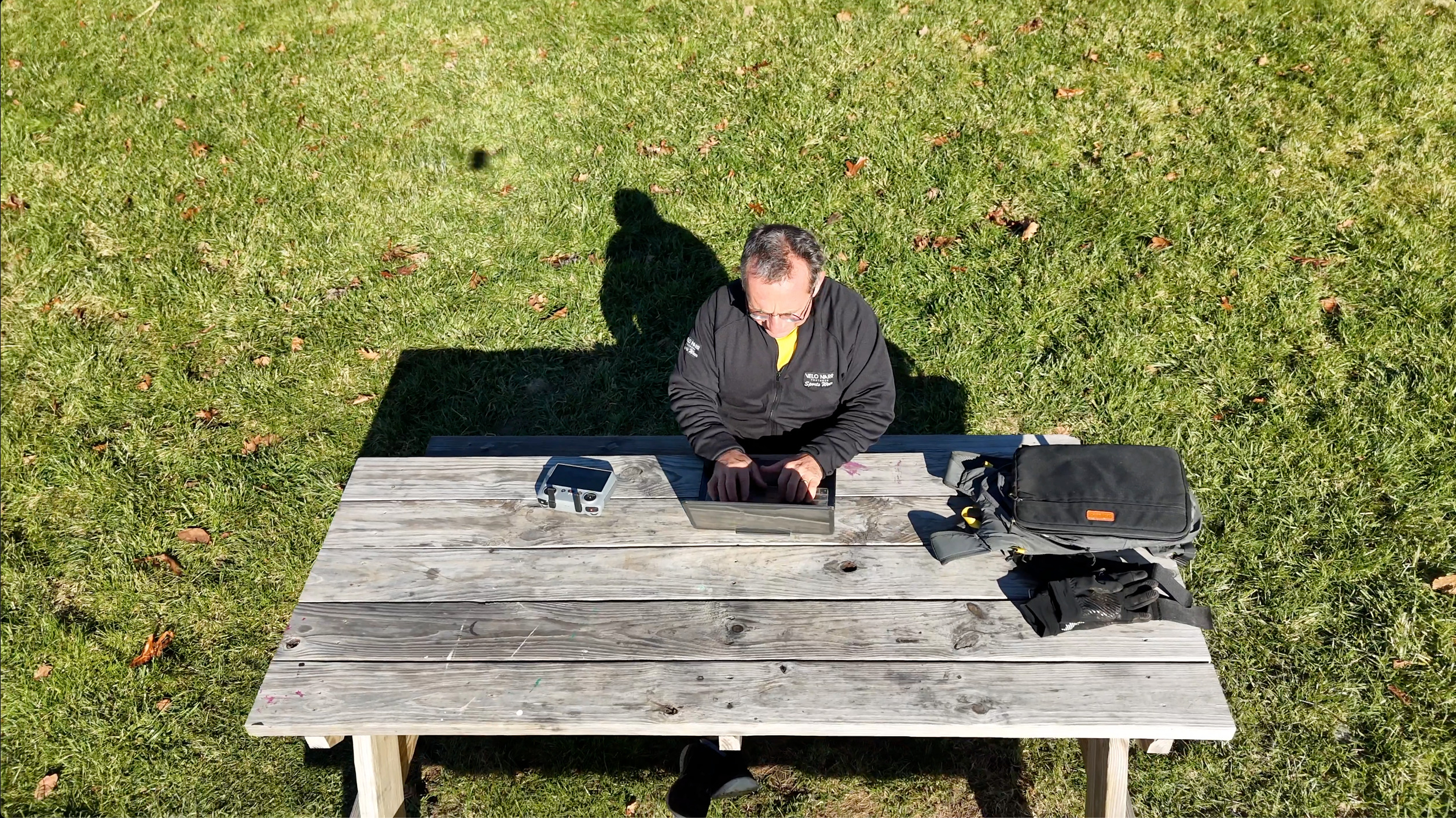
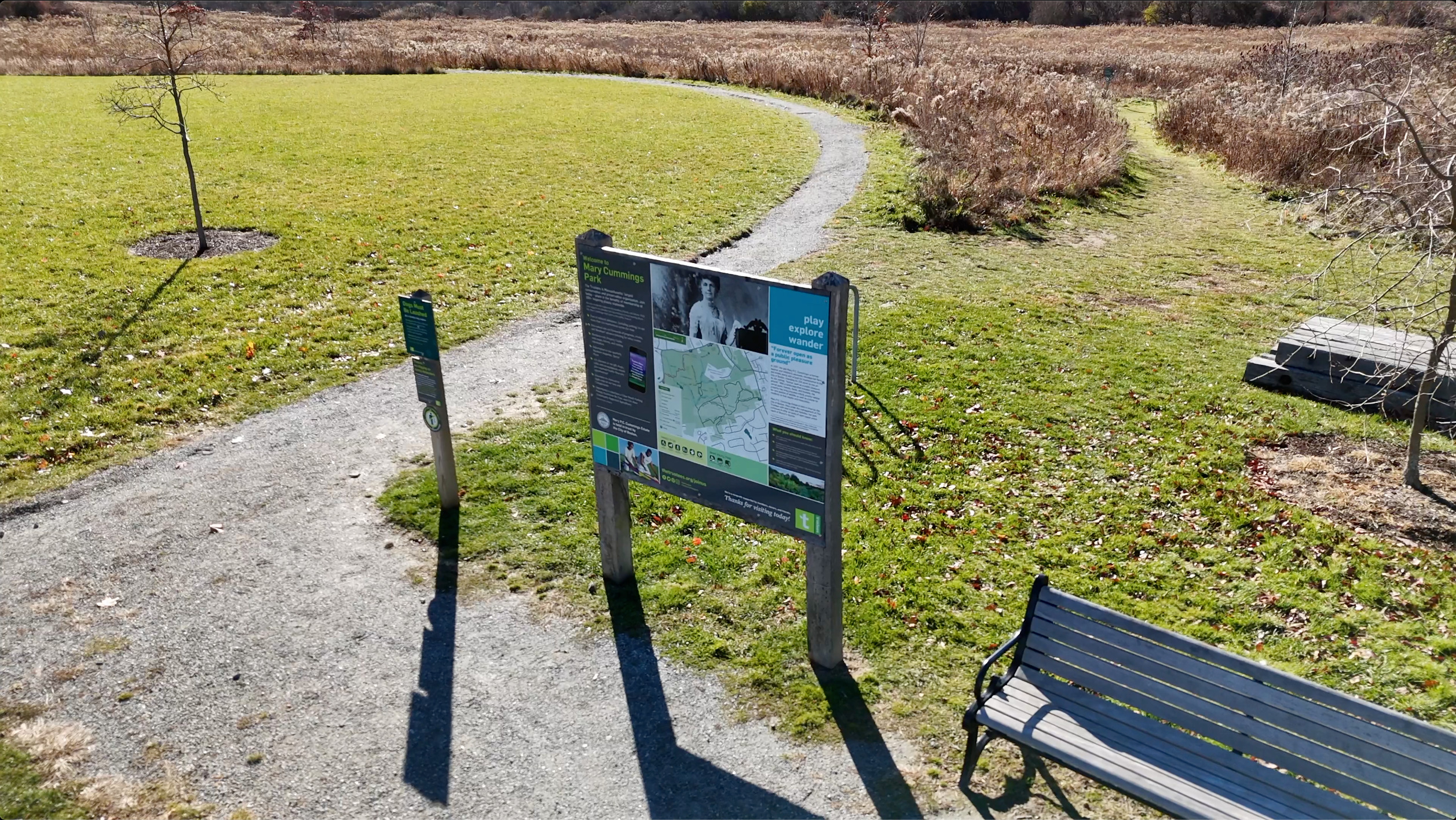
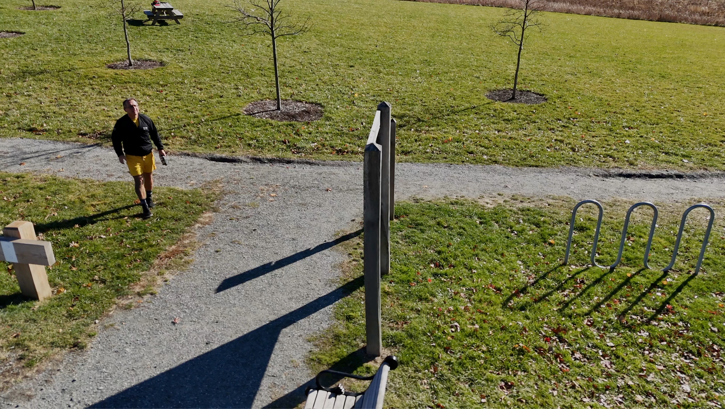
 The pictures at the beginning of the clip were done on Tuesday morning before thanksgiving. I took a detour from my morning commuting bike ride into Cambridge and instead of just directly going along Mass Avenue, passed first along the Mystic river, took out my Avata camera for a spin on a beach of the river and then continued the bike ride to Cambridge. It is a 10 minute detour (30 minutes instead of 20), but the Mystic river (like also the Mystic lakes) are very beautiful, especially in the morning. One can see the calm water and clear sky. Later in the day, the air and sky is usually much less clear and the waters usually less calm. The pictures after the presentation were taken during my thanksgiving run through the Mary Cummings park. We live in Arlington since 23 years. In the first few years, I had explored this area of Burlington mostly by bike or roller blades, but during the pandemic, it became one of my favorite running routes and it is since then stayed a favorite during weekends, where I have a bit more time and can spend 2 hours outside. From our house, I can reach the park in 45 minutes while running on a direct route. In colder months I like to run with my backpack and laptop in and take a break in the Starbucks at the West Cummings park (But I must admit that it was often also during the pandemic a favorite stop). One can see this Starbucks in some of the pictures below, I picked some frames from the clip, where my DJI mini had been visited by some birds. The West Cummings park Mall is usually quite busy, but during Thanksgiving (Thursday), essentially only the Starbucks was open. I like both the Mini 4 and the Avata cameras because they are so small. They easily pack into a small running backpack, even together with my mac-book air laptop and some additional thin running coat in case of rain. To do so, I stick the DJI mini into a sock and the Avata into a shirt before stuffing it into the back-back. When packing both drones, the laptop does not fit any more into the small running backback. For example, on yesterday’s Saturday afternoon after thanksgiving, I packed both drones for our traditional thanksgiving hike in Winchester.