The dyadic zeta story in a nutshell
[ Update: January 14, 2018: The paper on Elementary Dyadic Riemann Hypothesis [ArXiv] (see also local [PDF]) is a writeup of what is exposited here. ]
The Riemann zeta function is the spectral zeta function of the circle $T$, a topological group which is the Pontryagin dual of the group of the rational integers $Z$. We look here at the zeta function analogue, where the field of real numbers $R$ is replaced by the field of dyadic numbers $X$, where the group $Z$ is replaced with the Prüfer group $P$ and where the circle group $T$ is replaced with the dyadic group of integers $D$. The dyadic story is completely different from the real story. Unlike in the Riemann zeta function case, where the structure of the primes in Z is intricate and complicated, the Dyadic case is “integrable” in the sense that we know virtually everything about the zeta function. It reflects the fact that since the Prüfer group P is a divisible group (meaning that for every positive integer n, the group n P is the group P itself), there are no interesting primes. The Dyadic zeta function is now an explicitly known entire function satisfying a functional equation $\zeta(s)=\zeta(-s)$ which has all roots on the imaginary axes. This is a dyadic Riemann hypothesis. This story of the Dyadic zeta function tells nothing about the Riemann hypothesis. The Dyadic and Real worlds are far apart. It is an interesting analogy however and illustrates how natural the connection calculus is and how it is tied to a dyadic arithmetic.
[Update Jan 9: the statement that the classical and dyadic stories are “far apart” might have to be modified: a recent conjecture of Friedli and Karsson in the Hodge Laplacian case: if the approximation of the circular Hodge zeta function to the limiting zeta function of $Z$ is good enough in the critical strip, then the Riemann hypothesis holds. This amounts of estimating the integral of $f(x)=\sin^s(\pi x)$ with a Riemann sum on the interval $[0,\pi]$. In the dyadic case, we have also that the zeta functions of finite simplicial complexes are Riemann sums to an entire function. As the limiting zeta function is just a transplanted f, it is very likely that the same Friedkli-Karsson statement holds also for the Dyadic approximation. More about this in the last section of this blog entry.]
A functional equation
Mid December stroke the experimental discovery that for a one-dimensional finite abstract simplicial complex G, the spectrum of the connection Laplacian L [defined by $L(x,y)=1$ if $x \in G$ and $y \in G$ intersect and $L(x,y)=0$ if $x$ and $y$ are disjoint] satisfies the symmetry $\sigma(L^2) = \sigma(L^{-2})$. Talking about the inverse $L^{-1}$ makes sense because $g=L^{-1}$, the Green’s function operator is bounded by the unimodularity theorem. The functional equation is remarkable and was unexpected. It was undetected for so long because we usually look at higher dimensional or randomly generated complexes, which are most of the time not one-dimensional. An other reason why the result was a bit hidden as we have to get to used to the fact that the connection Laplacian is actually better an analogue of the Dirac operator and not of the Laplacian. Like in the Hodge case, where $H=D^2$ is the Hodge Laplacian defined by the Dirac operator $D=d+d^*$ (where $d$ is the exterior derivative in the form of incidence matrices defined by Poincaré) we should maybe think of the square $L^2$ as the right analogue of the Laplacian. Anyway, it is positive definite, like the classical Hodge Laplacian $H=D^2$ [which has a continuum analog in the form of differential operators] is positive semi-definite.
The spectral symmetry tells that for every eigenvalue $\lambda$ of the connection Laplacian $L$, there is an eigenvalue $\pm \lambda^{-1}$. This observation was only made after looking at the roots of the connection zeta function $\zeta(s)$ defined as $\sum_{k=1}^n (\lambda_k^2)^{-s/2}$, where $\lambda_k$ are the eigenvalues of $L$. The reason to normalize the zeta function and take $\zeta_{L^2}(s/2)$ rather than $\zeta_L(s)$ is because with negative $\lambda$, there is the ambiguity of choosing a root. As $L$ has both positive and negative spectrum, the pictures of the zeta function are just not nice. Taking the square of the operator and taking $s/2$ (even so the later division by 2 is often not done any more) normalizes the zeta function nicely. This is quite familiar as the Riemann zeta function is normalized in the same way when seeing it as the Zeta function of the Dirac operator $D=i d/dx$ on the circle $T=R/Z$. The Dirac operator $D$ on the circle has the eigenvalues $\lambda_n=-n$ with eigenvector $\phi_n(x)=\exp(i n x)$ but $\sum_{n \in Z} n^{-s}$ does not work well at all. It is better to take the positive eigenvalues $n^2$ of the Laplacian $D^2=-d^2/dx^2$ to get the familiar definition $\sum_{n \geq 1} n^{-s}$. The eigenvalue $0$ of the Dirac operator belonging to the constant function is ignored in the Riemann zeta function case. This reflects the fact that in differential geometry, the zeta regularized determinant is actually a Pseudo determinant and not a determinant. Zeta regularizations of determinants and spanning tree formulas are a major motivation to study pseudo determinants and more generally the coefficients of the characteristic polynomial and not only determinants, which is one particular coefficient of the characteristic polynomial. In the connection operator case, we don’t need to ignore the zero eigenvalue as $L$ is always invertible.
| Theorem (Functional equation). The connection zeta function $\zeta(s)$ of any one-dimensional simplicial complex satisfies the functional equation $\zeta(s)=\zeta(-s)$. |
The functional equation is equivalent to the fact that the spectrum of $L$ satisfies the symmetry $\sigma(L)=1/\sigma(L)$. It is also equivalent to the statement that the characteristic polynomial of $L^2$ is palindromic. For general complexes the spectrum does not satisfy this symmetry. It is a feature however for one-dimensional complexes. By the way, we so far have not seen a two or higher dimensional simplicial complex which has this spectral symmetry. The palindromic property might characterize complexes which have dimension 0 or 1 but we have not thought about this theoretically yet.
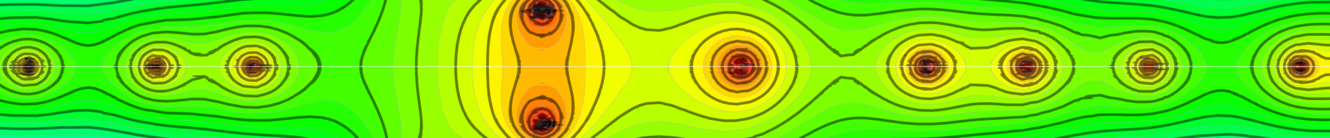
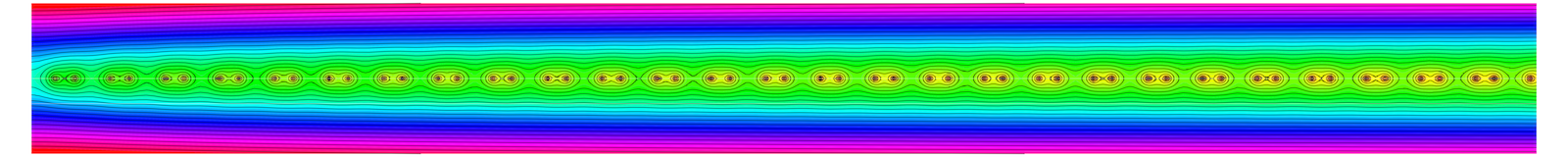
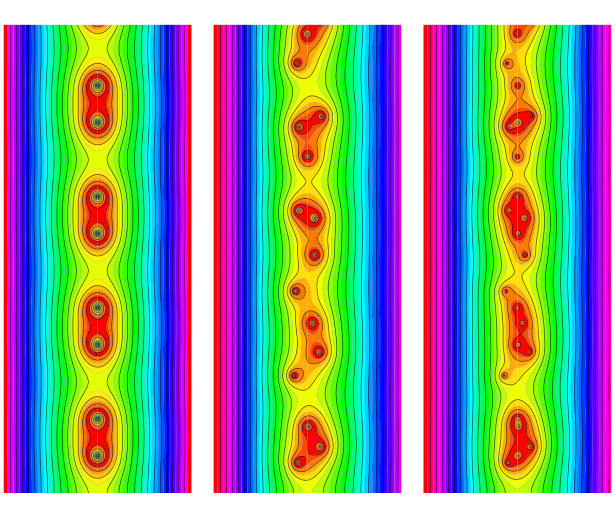
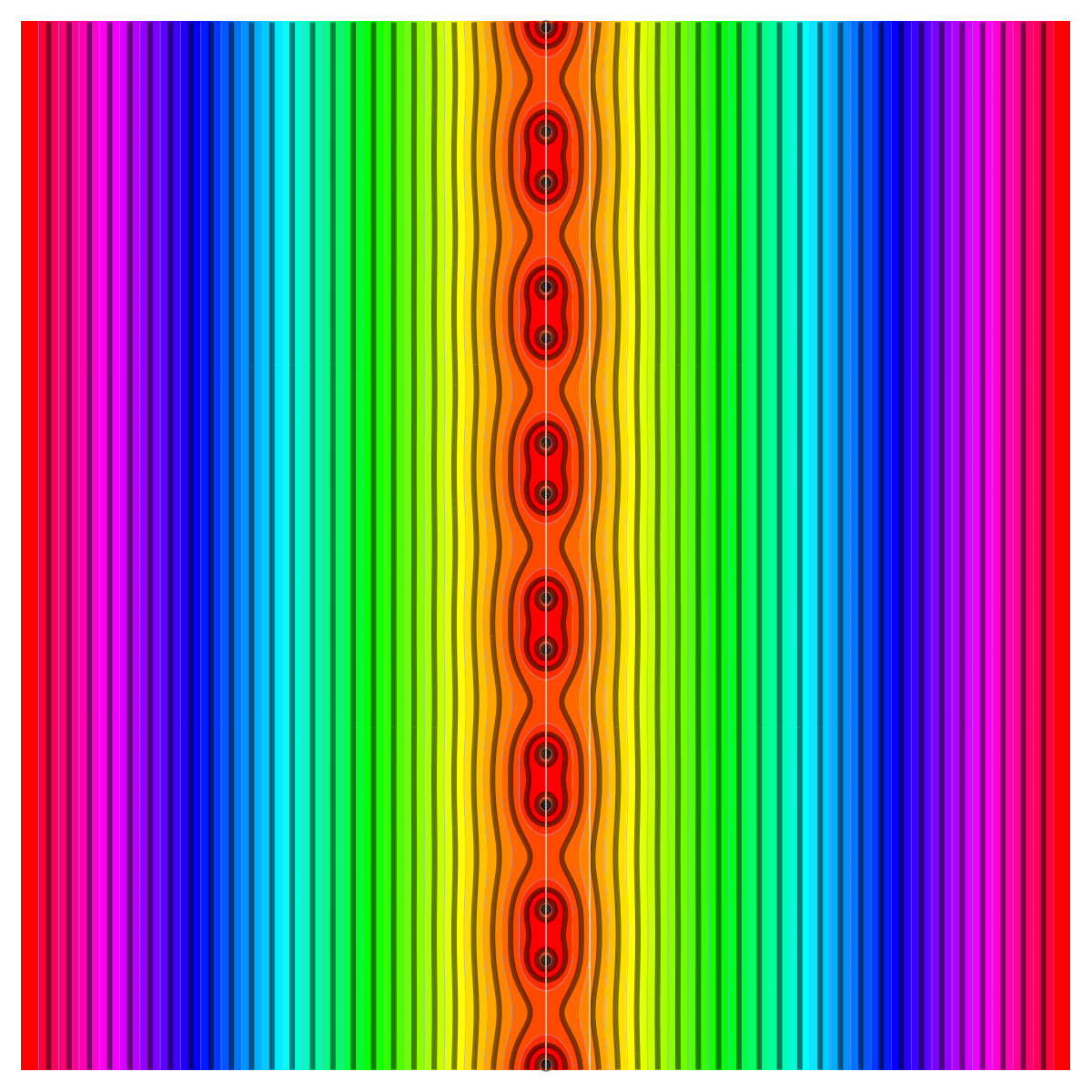
Here is a picture of a zeta function of a one dimensional simplicial complex. It has been rotated so that the imaginary axes is the horizontal axes and so that the real axes is at the center pointing north. The picture shows the level curves of the zeta function of the one-dimensional figure 8 complex, a graph with 7 vertices, 8 edges, Betti numbers $b_0=1, b_1=2$. We see clearly the spectral symmetry.
The figure 8 graph is a one-dimensional simplicial complex with Euler characteristic 7-8=-1. The eigenvalues of the square of the connection Laplacian $L^2$ are $\{0.0319675, 0.0736202, 0.116692, 0.171573, 0.171573, 0.561177, 1., 1., 1., 1.78197, 5.82843, 5.82843, 8.5696, 13.5832, 31.2817\}$. The spectral symmetry can be observed by seeing that if $\lambda$ is an eigenvalue, then also $1/\lambda$ is an eigenvalue of $L^2$.
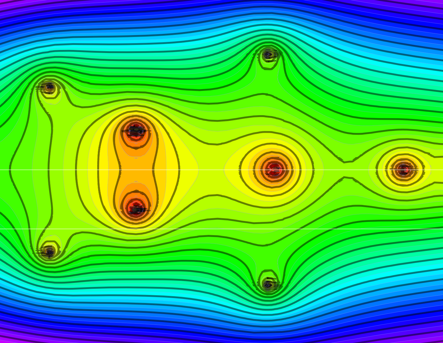
Lets look at an other zeta function picture. It belongs to the triangle graph, which is a two-dimensional simplicial complex of Euler characteristic 3-3+1=1. The spectrum of the $7×7$ squared connection matrix $L^2$ is $\{30.3756, 2.61803, 2.61803, 0.566283, 0.381966, 0.381966, 0.0581356\}$. There is no spectral symmetry. Indeed, the complex is no more one-dimensional. Here is a picture of the level curves of the zeta function. Again the picture turned so that the imaginary axes looks to the right and the real axes points upwards. We see that the functional equation does not hold any more:
The Dyadic Riemann hypothesis
The Dyadic group of integers D is not as familiar to us than the circle T. It is a much simpler space however as it is completely disconnected and is quantized, (we have a smallest translation in D, defining a dynamical system which is also called the “adding machine”), it is still a compact space and a natural limit of one-dimensional geometric spaces in the Barycentric limit. The Pontryagin dual P of D, the Prüfer group, does not have any interesting primes. The Prüfer group is the spectrum of the Koopman operator of the adding machine. I originally had been led to this via ergodic theory, when looking at renormalizations of random Jacobi matrices. The Dyadic group appeared there naturally as a limit of a 2:1 integral extension in ergodic theory: the group translation is called the von Neumann-Kakutani system. The 2:1 integral extension is probably the most simple “renormalization map” as it is a simple contraction in the complete metric space of measure preserving dynamical systems. One can reverse the map by looking at the return map onto the original part of the probability space squaring the map. Its unique fixed point is integrable, a group translation on D.
The limiting operators are almost periodic operators defined over that ergodic system. The spectra are located on Julia sets, the density of states are the equilibrium measures on that sets. In some sense, these Jacobi operators define a “quantization of the concept of Julia sets” as they are operators for which the spectra are Julia sets. In some sense by looking at Barycentric refinements of simplicial complexes, we introduce in the limit a system which has this scaling symmetry.
Some other mathematical connections to the dyadic world are discussed here, in a blog of Tao from more than 10 years ago where the importance of dyadic models is stressed like: (citation: Very broadly speaking, one of the key advantages that dyadic models offer over non-dyadic models is that they do not have any “spillover†from one scale to the next.) Our angle is more simplistic: we compare the real world and dyadic world by looking at the properties of the underlying spaces:
| Object/Property | Real world | Dyadic world |
|---|---|---|
| Field | Real line | Dyadic numbers X |
| Topological group | Circle T | Dyadic group D | Pontryagin dual | Integers Z | Prüfer group P |
| Divisibility | T is divisible | P is divisible |
| Compactness | T is compact | D is compact |
| Connectedness | T is | Neither D nor P |
| Profinite | Neither T nor Z | D is profinite |
| Smallest translation | Z has | D has smallest translation step |
| Quotient | T=R/Z | P=X/D |
| Laplacian | $D^2=-d^2/dx^2$ | $L^2$ |
| Zeta function | Riemann zeta function | limit of $\zeta(C(2^n))$ |
| Feels like | Classical | Quantum |
The lack of interesting primes in the Prüfer group manifests when looking at the zeta function in the Barycentric limit:
| Theorem (Dyadic Riemann Hypothesis). For any one-dimensional simplicial complex $G$, the rescaled zeta functions $\zeta_{G_n}/|G_n|$ of the successive Barycentric refinements $G_n$ of $G$converge to an entire function which has all roots on the imaginary axes and satisfies the functional equation $\zeta(s)=\zeta(-s)$. |
An explicit formula for the limiting zeta function is
$$ z(it) = \int_0^1 \frac{2 \cos(2 t \log(\sqrt{4 v^2+1}+2 v))}{\pi \sqrt{1-v} \sqrt{v}} \, dv \; . $$
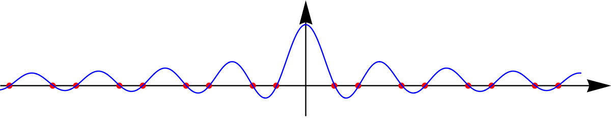
We wrote it with the rotated variable $s=it$ so that for real $t$, we get a real function. Her is the graph of that real function. The roots are the roots of the zeta function.
[We tried to relate the integral in terms of known functions like some kind of hyperelliptic function but had no luck so far. Computer algebra systems are usually quite good in figuring out such connections. The integral looks a bit complicated but it is actually just the conformal image of the equilibrium measure on an interval under a Joukowski type map $S(z)=z-1/z$. There is no “meta law” which assures that simple natural expressions need to have a name. The pendulum system or the Kepler problem are both cases where basic elementary functions do not catch any more and elliptic integrals appear. Still, it could well be that the integral can be expressed in terms of some hyperelliptic functions, we just did not find it yet. But here are two Mathematica expression before and after a trig substitution
Integrate[ 2*Cos[2t*Log[(2*Sin[Pi*x]^2 + Sqrt[1 + 4*Sin[Pi*x]^4])]],{x,0,1}]
Integrate[ 4*Cos[2t*Log[2*v+Sqrt[1+4*v^2]]]/(2 Sqrt[v] Pi Sqrt[1-v]),{v,0,1}]
]
We had proven an other Baby Riemann hypothesis for the Hodge operators $H=D^2$ of a simplicial complex. What happened there is that the limiting roots are on the axes Re(s)=1. But there, no explicit formula for the limiting zeta function is found yet. The proof in the Hodge case was much harder and more technical as there was no functional equation. It required to analyze the situation in three different regions of the complex plane. In one region, the analysis was similar to what happens in the connection graph, on a second region Re(s)>1, there had been a connection with the Riemann zeta function. Then, in the critical strip, the analysis required some subtle single variable calculus. Here, in the connection Laplacian case, the analysis is straightforward as we will see below.
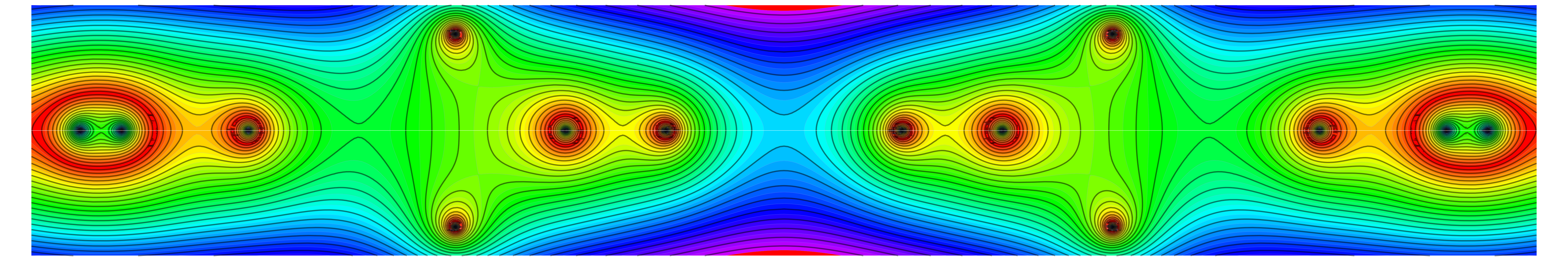
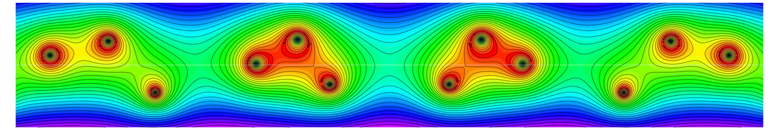
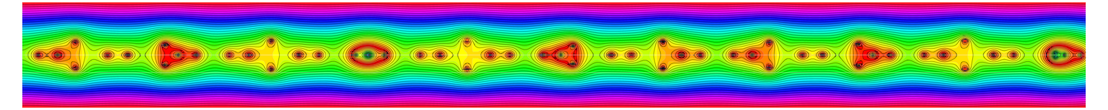
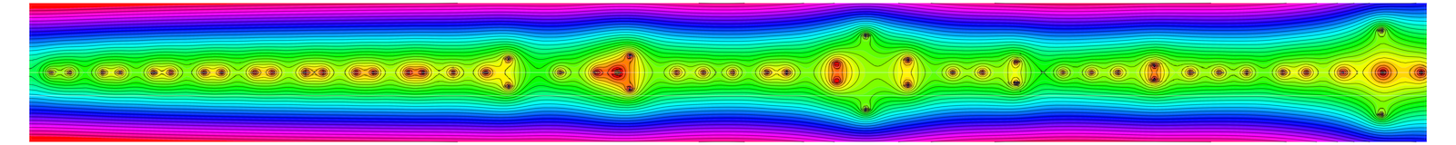
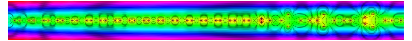
The convergence happens for example uniformly on compact subsets of the complex s-plane. We will in the next section explain a bit the proof. Let us look at some pictures of Zeta functions for circular graphs. We first see the circular graph with 4 vertices, then with 32 vertices, 64 and finally with 128 vertices, where we are already very close to the limiting zeta function. In all four pictures, the real axes points upwards and is on the left hand side of the picture (we only show part of the upper half plane as the picture to the left looks the same).
|
|
|
|
Elements of the proof
While the mathematics is pretty explicit, there are still some interesting pieces in the proof.
A) PYTHAGORAS We can make use of our generalized Cauchy-Binet formula for arbitrary $n \times m$ matrices $F,G$. It tells that the $k$’th coefficient of the characteristic polynomial of the $m \times m$ square matrix $F^T G$ is an interior product $p_k(F^T G) = \sum_{|P|=k} {\rm det}(F_P) {\rm det}(G_P)$ of minors. The classical Cauchy-Binet case is the special case of the largest coefficient $p_m$. The product formula for determinants is the case when both F and G are square matrices. We first had generalized that Cauchy-Binet to pseudo determinants which is the largest non-zero $p_k$ and then extended it to all characteristic polynomials. [By the way, the literature on determinants is huge and in that research in a very classical area, more time was spent to check that the result is really new and not hidden in some publication. There are other special cases which are known like the case $k=1$ (for which $p_1$ is the trace), and where the identity is a Hilbert-Schmidt identity). Also for square matrices F=G, one can see the result as a trace formula used in functional analysis (especially in the context of Trace ideals) and Fredholm determinants. [By the way, my own exposure in this matter had been sharpened in mathematical physics, especially by attending a course of Barry Simon on trace ideals (around 1995).]
B) PALINDROMS An other ingredient in the proof is to give explicit formulas for the eigenvalues of the connection Laplacians for circular graphs. Unlike the Hodge case, where Fourier theory directly diagonalizes the matrices, we had to fight for a while for explicit formulas in that case. I only managed to get this at the very end of the old year 2017 after two days of experientation. It turns out that we have to make a nonlinear coordinate transformation in order to use Fourier theory. It is obvious, once seen but not needed detours over palindromic polynomials to get to it. What led to the idea is that every unimodular palindromic polynomial can be expressed using a polynomial of half the degree and that that this is the characteristic polynomial of an other operator. It is in some sense a nonlinear renormalization map in the space of palindromic polynomials. Palindromic polynomials appear to be related to recreational mathematics but they are important in virtually any part of mathematics! The Alexander polynomials of knots for example are palindromic. We even looked once at palindromic Schroedinger operators even so there, the potentials of the operators and not the characteristic polynomials were palindromic.
C) RIEMANN SUMS A third ingredient is borrowed from the Hodge case paper. It deals with the elementary (but very exciting) story of Riemann sums of a smooth function. That story is certainly not to the taste of contemporary mathematics (which loves complexity) but it is close to what we teach to undergraduates and where mathematics is most fun, as one can see everything with crystal clear clarity and understand. What happens if we take a smooth function $f$ on the interval $[0,1]$ an compare the Riemann sum $S(n)=\sum_{k=1}^n f(k/n)$ with the integral $S=\int_0^1 f(x) \; dx$? Of course $S(n)/n$ converges to $S$, but how fast. It happens surprisingly fast. We can even estimate $S(n)-n S$ using higher derivatives. Now, it turns out that Zeta functions (both in the Hodge as well as in the connection case) are Riemann sums of explicitly known functions. This allows us to analyze the convergence.
D) BARYCENTRIC LIMITS An other old story comes in as we want to see that the limiting zeta function does not depend on the starting complex. This requires to estimate the eigenvalues of complexes which have undergone surgery. For one-dimensional complexes this is particularly simple. We have only to cut and reglue the complex at finitely many vertices to get a circular graph. And the number of cuts and gluings does not depend on the stage of the Barycentric refinement at all. A basic theorem of Lidsky (again a linear algebra story) allows now to see the difference between the zeta functions. This is also an older story see here. See also this presentation on slides explaining the central limit theorem (convergence of the density of states in law) in that case.
In the next few sections, we plan to say more in each case. A document with a write up will appear soon.
The Euler characteristic in terms of the Zeta function
Before we look at the proof, let us look at two formulas which illustrate how we got to the zeta function from previous investigations. There is more information in the non-normalized zeta function $\sum_{k=1}^n \lambda_k^{-s}$, where $\lambda_k$ are the eigenvalues of the connection Laplacian $L$ of a finite abstract simplicial complex $G$. We don’t assume here that G is one-dimensional. We first of all have $\zeta_L'(0) = -i \pi n(G)$, where $n(G)$ is the number of negative eigenvalues. The unimodularity theorem $|{\rm det}(L)|=1$ implies ${\rm Re}( \log(L) )= 0$. Now, ${\rm Im}(\log(L)) = i\pi (n(G))$, where $n(G)$ is the number of negative eigenvalues. The fact that $n(G)$ is the number of odd-dimensional simplices (the Morse index if we think of L as a Hessian matrix) was proven before. But now we can express the Euler characteristic in terms of the zeta function: $\chi(G) = \zeta(0)-2 i \zeta'(0)/\pi$. The reason is that $\zeta(0)=p(G)+n(G)$ and $i \zeta'(0)/\pi = n(G)$ so that $\chi(G)=p(G)-n(G) = \zeta(0)-2 i \zeta'(0)/\pi$. Also the determinant of $L$ can be expressed in terms of the Zeta function: $(-1)^{n(G)} = \exp(-i \zeta’_L(s)) = {\rm det}(L(G))$. These formulas hold in general. We will look more about cohomology of a complex from the spectrum but as we have seen already that only works for subclasses of complexes: there are even one-dimensional examples of complexes for which isospectral complexes have different cohomology.
The functional equation
|
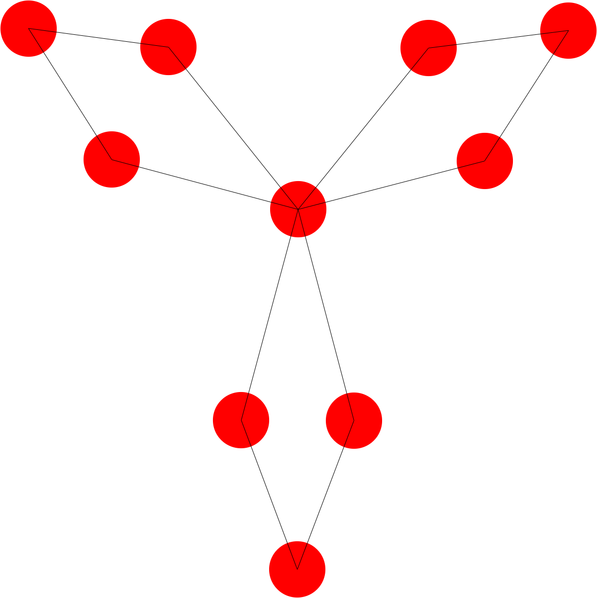
To prove the functional equation, we need to show the palindromic property $p_k = p_{n-k}$. We use the notation $p(x) = {\rm det}(A-x I) = p_0(-x)^n +p_1(-x)^{n-1} + \dots +p_k(-x)^{n-k} + \dots + p_n$ for the characteristic polynomial of a matrix $A$. Here is an example: we take a 3-clover graph, which is a one-dimensional sphere bouquet with three leaves. It has the f-vector (10,12) and 10+22 22 simplices and Euler characteristic $10-12=-2 = b_0-b_1=1-3$. The genus $1-\chi(G)$ counts the number of holes in a one-dimensional complex. We have seen in various places that the genus $1-\chi(G)$ plays an important role everywhere else, also in higher dimensions. The diagonal entries $g(x,x)$ of the Green function $g=L^{-1}$ for example is given as the genus of the unit sphere $S(x)$. The Poincaré-Hopf index of a locally injective function $f$ is defined as the genus of the stable sphere $S^-(x)=\{ y \in S(x) | f(y) < f(x) \}$. The sum over all the genus values of the unit spheres of a complex is the trace of the Hydrogen operator, which will play a role in a second. |
The connection Laplacian is the $22 \times 22$ matrix
$$ L=\left[ \begin{array}{cccccccccccccccccccccc}
1&0&0&0&0&0&0&0&0&0&1&1&1&1&1&1&0&0&0&0&0&0\\
0&1&0&0&0&0&0&0&0&0&1&0&0&0&0&0&1&0&0&0&0&0\\
0&0&1&0&0&0&0&0&0&0&0&0&0&0&0&0&1&1&0&0&0&0\\
0&0&0&1&0&0&0&0&0&0&0&1&0&0&0&0&0&1&0&0&0&0\\
0&0&0&0&1&0&0&0&0&0&0&0&1&0&0&0&0&0&1&0&0&0\\
0&0&0&0&0&1&0&0&0&0&0&0&0&1&0&0&0&0&0&1&0&0\\
0&0&0&0&0&0&1&0&0&0&0&0&0&0&0&0&0&0&1&1&0&0\\
0&0&0&0&0&0&0&1&0&0&0&0&0&0&1&0&0&0&0&0&1&0\\
0&0&0&0&0&0&0&0&1&0&0&0&0&0&0&0&0&0&0&0&1&1\\
0&0&0&0&0&0&0&0&0&1&0&0&0&0&0&1&0&0&0&0&0&1\\
1&1&0&0&0&0&0&0&0&0&1&1&1&1&1&1&1&0&0&0&0&0\\
1&0&0&1&0&0&0&0&0&0&1&1&1&1&1&1&0&1&0&0&0&0\\
1&0&0&0&1&0&0&0&0&0&1&1&1&1&1&1&0&0&1&0&0&0\\
1&0&0&0&0&1&0&0&0&0&1&1&1&1&1&1&0&0&0&1&0&0\\
1&0&0&0&0&0&0&1&0&0&1&1&1&1&1&1&0&0&0&0&1&0\\
1&0&0&0&0&0&0&0&0&1&1&1&1&1&1&1&0&0&0&0&0&1\\
0&1&1&0&0&0&0&0&0&0&1&0&0&0&0&0&1&1&0&0&0&0\\
0&0&1&1&0&0&0&0&0&0&0&1&0&0&0&0&1&1&0&0&0&0\\
0&0&0&0&1&0&1&0&0&0&0&0&1&0&0&0&0&0&1&1&0&0\\
0&0&0&0&0&1&1&0&0&0&0&0&0&1&0&0&0&0&1&1&0&0\\
0&0&0&0&0&0&0&1&1&0&0&0&0&0&1&0&0&0&0&0&1&1\\
0&0&0&0&0&0&0&0&1&1&0&0&0&0&0&1&0&0&0&0&1&1\\
\end{array} \right] \; . $$
The coefficients $p_k$ of the characteristic polynomial are the palindrome $\{1, 118, 5199, 121460, 1725515, 15972510, 100208325, 436757040, 1345933002, 2974271212, 4764416470$,
$5570332344$, $4764416470, 2974271212, 1345933002, 436757040, 100208325, 15972510, 1725515, 121460, 5199, 118, 1\}$. The eigenvalues of $L^2$ are
$54.3423, 13.5832, 13.5832, 9.53444, 5.82843, 5.82843, 5.82843, 1.78197, 1.78197, 1., 1.$, $1., 1., 0.561177, 0.561177, 0.171573, 0.171573, 0.171573, 0.104883, 0.0736202, 0.0736202, 0.0184019$. We see the spectral symmetry $\sigma(L)=1/\sigma(L)$.
In order to prove the symmetry $p_k = p_{n-k}$, we use
| Generalized Cauchy-Binet formula: Given two arbitrary $n \times m$ matrices $F,G$. The coefficient $p_k$ of the Characteristic polynomial of $F^T G$ satisfy $p_k = \sum_P det(F_P G_P)$. |
Cauchy-Binet is the special case when $k=min(m,n)$ which gives $det(F^T G) = \sum_{|P|=k} det(F_P) G(P)$ and which is in the case $n=m$ the product formula $det(F G) = det(F) det(G)$ for determinants. As a special case, the coefficients $p_k$ of $L^2$ satisfy a Pythagorean identity
| Corollary (Generalized Pythagoras) Given a selfadjoint matrix L, then $p_k(L^2) = \sum_{|P|=k} det(L_P)^2$ |
A special case of that is the Hilbert-Schmidt identity $tr(L^2) = \sum L_{ij}^2$ which already generalizes Pythagoras and justifies the name. To prove the functional equation, we have to show that $p_k = p_{n-k}$. The above Pythagorean formula reduces this to a question about determinants. The proof then goes by induction but as we have to track not only determinants but all coefficients of the characteristic polynomial during the deformation, we need a bit more analysis. Of course we hoped to find an interpolating deformation of the operators such that $p_k(t)-p_{n-k}(t)$ remains zero. This hope was in vain and the obstacle was overcome only when the fall semester was over and I had more time. During the interpolating deformation $p_k(t)-p_{n-k}(t)$ is not zero! If we use the deformation like in the this paper when proving the spectral formula $\chi(G) = p(G)-n(G)$, where $p(G)$ is the number of positive eigenvalues and $n(G)$ the number of negative eigenvalues. But there is a miracle happening: if we deform the Laplacian when adding a new cell, then we can look at $\phi_k(t) = p_k(t)-p_{n-k}(t)$. It would have been simplest if $\phi_k(t)$ remained zero. But it does not! We therefore have to track the motion. The differential equation for the quadratic functions in $t$ and prove that $\phi_k(t)=0$ for $t=0$ and $t=1$.
The spectrum in the circular case
Let G be the circular graph $C_n=C_8$. Its Whitney complex is = $\{\{1\},\{2\},\{3\},\{4\},\{5\},\{6\},\{7\},\{8\},\{1,2\},\{1,8\},\{2,3\},\{3,4\},\{4,5\},\{5,6\},\{6,7\},\{7,8\}\}$. Lets look first at the Dirac operator $D$ which is
$$
D = \left[
\begin{array}{cccccccccccccccc}
0 & 0 & 0 & 0 & 0 & 0 & 0 & 0 & -1 & -1 & 0 & 0 & 0 & 0 & 0 & 0 \\
0 & 0 & 0 & 0 & 0 & 0 & 0 & 0 & 1 & 0 & -1 & 0 & 0 & 0 & 0 & 0 \\
0 & 0 & 0 & 0 & 0 & 0 & 0 & 0 & 0 & 0 & 1 & -1 & 0 & 0 & 0 & 0 \\
0 & 0 & 0 & 0 & 0 & 0 & 0 & 0 & 0 & 0 & 0 & 1 & -1 & 0 & 0 & 0 \\
0 & 0 & 0 & 0 & 0 & 0 & 0 & 0 & 0 & 0 & 0 & 0 & 1 & -1 & 0 & 0 \\
0 & 0 & 0 & 0 & 0 & 0 & 0 & 0 & 0 & 0 & 0 & 0 & 0 & 1 & -1 & 0 \\
0 & 0 & 0 & 0 & 0 & 0 & 0 & 0 & 0 & 0 & 0 & 0 & 0 & 0 & 1 & -1 \\
0 & 0 & 0 & 0 & 0 & 0 & 0 & 0 & 0 & 1 & 0 & 0 & 0 & 0 & 0 & 1 \\
-1 & 1 & 0 & 0 & 0 & 0 & 0 & 0 & 0 & 0 & 0 & 0 & 0 & 0 & 0 & 0 \\
-1 & 0 & 0 & 0 & 0 & 0 & 0 & 1 & 0 & 0 & 0 & 0 & 0 & 0 & 0 & 0 \\
0 & -1 & 1 & 0 & 0 & 0 & 0 & 0 & 0 & 0 & 0 & 0 & 0 & 0 & 0 & 0 \\
0 & 0 & -1 & 1 & 0 & 0 & 0 & 0 & 0 & 0 & 0 & 0 & 0 & 0 & 0 & 0 \\
0 & 0 & 0 & -1 & 1 & 0 & 0 & 0 & 0 & 0 & 0 & 0 & 0 & 0 & 0 & 0 \\
0 & 0 & 0 & 0 & -1 & 1 & 0 & 0 & 0 & 0 & 0 & 0 & 0 & 0 & 0 & 0 \\
0 & 0 & 0 & 0 & 0 & -1 & 1 & 0 & 0 & 0 & 0 & 0 & 0 & 0 & 0 & 0 \\
0 & 0 & 0 & 0 & 0 & 0 & -1 & 1 & 0 & 0 & 0 & 0 & 0 & 0 & 0 & 0 \\
\end{array}
\right] $$
The Laplacian $L=D^2$ is
$$ H=D^2 = \left[
\begin{array}{cccccccccccccccc}
2 & -1 & 0 & 0 & 0 & 0 & 0 & -1 & 0 & 0 & 0 & 0 & 0 & 0 & 0 & 0 \\
-1 & 2 & -1 & 0 & 0 & 0 & 0 & 0 & 0 & 0 & 0 & 0 & 0 & 0 & 0 & 0 \\
0 & -1 & 2 & -1 & 0 & 0 & 0 & 0 & 0 & 0 & 0 & 0 & 0 & 0 & 0 & 0 \\
0 & 0 & -1 & 2 & -1 & 0 & 0 & 0 & 0 & 0 & 0 & 0 & 0 & 0 & 0 & 0 \\
0 & 0 & 0 & -1 & 2 & -1 & 0 & 0 & 0 & 0 & 0 & 0 & 0 & 0 & 0 & 0 \\
0 & 0 & 0 & 0 & -1 & 2 & -1 & 0 & 0 & 0 & 0 & 0 & 0 & 0 & 0 & 0 \\
0 & 0 & 0 & 0 & 0 & -1 & 2 & -1 & 0 & 0 & 0 & 0 & 0 & 0 & 0 & 0 \\
-1 & 0 & 0 & 0 & 0 & 0 & -1 & 2 & 0 & 0 & 0 & 0 & 0 & 0 & 0 & 0 \\
0 & 0 & 0 & 0 & 0 & 0 & 0 & 0 & 2 & 1 & -1 & 0 & 0 & 0 & 0 & 0 \\
0 & 0 & 0 & 0 & 0 & 0 & 0 & 0 & 1 & 2 & 0 & 0 & 0 & 0 & 0 & 1 \\
0 & 0 & 0 & 0 & 0 & 0 & 0 & 0 & -1 & 0 & 2 & -1 & 0 & 0 & 0 & 0 \\
0 & 0 & 0 & 0 & 0 & 0 & 0 & 0 & 0 & 0 & -1 & 2 & -1 & 0 & 0 & 0 \\
0 & 0 & 0 & 0 & 0 & 0 & 0 & 0 & 0 & 0 & 0 & -1 & 2 & -1 & 0 & 0 \\
0 & 0 & 0 & 0 & 0 & 0 & 0 & 0 & 0 & 0 & 0 & 0 & -1 & 2 & -1 & 0 \\
0 & 0 & 0 & 0 & 0 & 0 & 0 & 0 & 0 & 0 & 0 & 0 & 0 & -1 & 2 & -1 \\
0 & 0 & 0 & 0 & 0 & 0 & 0 & 0 & 0 & 1 & 0 & 0 & 0 & 0 & -1 & 2 \\
\end{array}
\right] \; $$
which consists of two copies $H_0,H_1$ of the Kirchhoff operator. Fourier theory diagonalizes the matrix. The eigenvalues are $2-2 \cos(2\pi k/n) = 4 \sin^2(\pi k/n)$. Now lets look at the connection Laplacian L which is defined as the matrix where $L(x,y)=1$ if the two simplices x,y intersect and $L(x,y)=0$ if they don’t intersect. The matrix is
$$L= \left[
\begin{array}{cccccccccccccccc}
1 & 0 & 0 & 0 & 0 & 0 & 0 & 0 & 1 & 1 & 0 & 0 & 0 & 0 & 0 & 0 \\
0 & 1 & 0 & 0 & 0 & 0 & 0 & 0 & 1 & 0 & 1 & 0 & 0 & 0 & 0 & 0 \\
0 & 0 & 1 & 0 & 0 & 0 & 0 & 0 & 0 & 0 & 1 & 1 & 0 & 0 & 0 & 0 \\
0 & 0 & 0 & 1 & 0 & 0 & 0 & 0 & 0 & 0 & 0 & 1 & 1 & 0 & 0 & 0 \\
0 & 0 & 0 & 0 & 1 & 0 & 0 & 0 & 0 & 0 & 0 & 0 & 1 & 1 & 0 & 0 \\
0 & 0 & 0 & 0 & 0 & 1 & 0 & 0 & 0 & 0 & 0 & 0 & 0 & 1 & 1 & 0 \\
0 & 0 & 0 & 0 & 0 & 0 & 1 & 0 & 0 & 0 & 0 & 0 & 0 & 0 & 1 & 1 \\
0 & 0 & 0 & 0 & 0 & 0 & 0 & 1 & 0 & 1 & 0 & 0 & 0 & 0 & 0 & 1 \\
1 & 1 & 0 & 0 & 0 & 0 & 0 & 0 & 1 & 1 & 1 & 0 & 0 & 0 & 0 & 0 \\
1 & 0 & 0 & 0 & 0 & 0 & 0 & 1 & 1 & 1 & 0 & 0 & 0 & 0 & 0 & 1 \\
0 & 1 & 1 & 0 & 0 & 0 & 0 & 0 & 1 & 0 & 1 & 1 & 0 & 0 & 0 & 0 \\
0 & 0 & 1 & 1 & 0 & 0 & 0 & 0 & 0 & 0 & 1 & 1 & 1 & 0 & 0 & 0 \\
0 & 0 & 0 & 1 & 1 & 0 & 0 & 0 & 0 & 0 & 0 & 1 & 1 & 1 & 0 & 0 \\
0 & 0 & 0 & 0 & 1 & 1 & 0 & 0 & 0 & 0 & 0 & 0 & 1 & 1 & 1 & 0 \\
0 & 0 & 0 & 0 & 0 & 1 & 1 & 0 & 0 & 0 & 0 & 0 & 0 & 1 & 1 & 1 \\
0 & 0 & 0 & 0 & 0 & 0 & 1 & 1 & 0 & 1 & 0 & 0 & 0 & 0 & 1 & 1 \\
\end{array}
\right] $$
Can we find an explicit expression for the eigenvalues? Fourier theory does not do it any more.
A few spectra
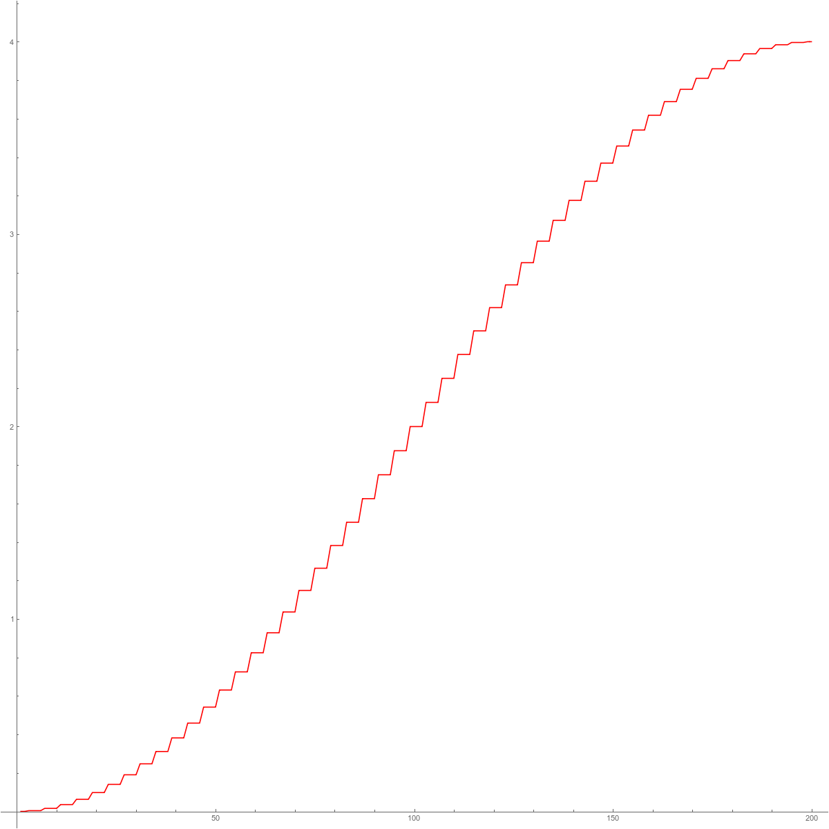
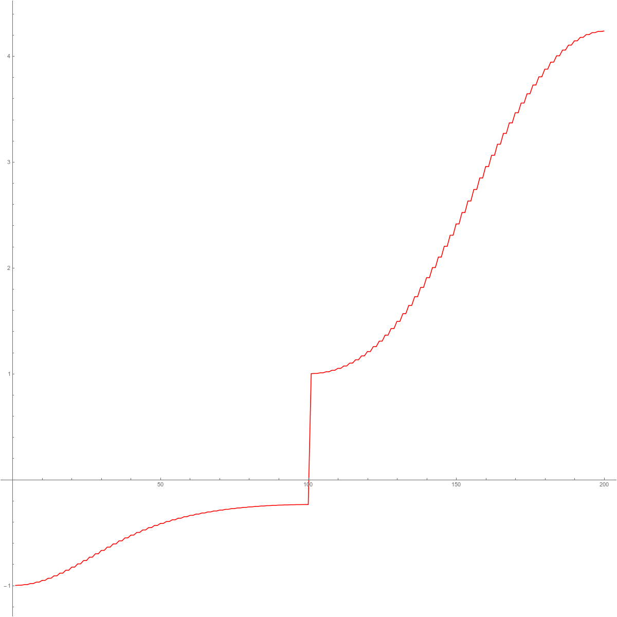
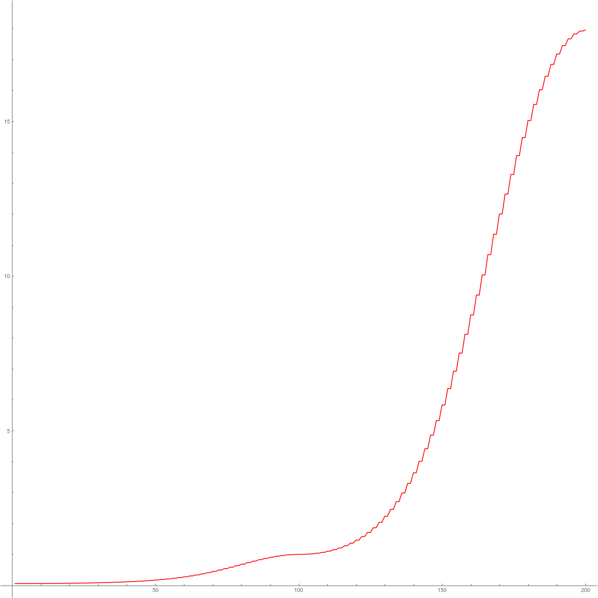
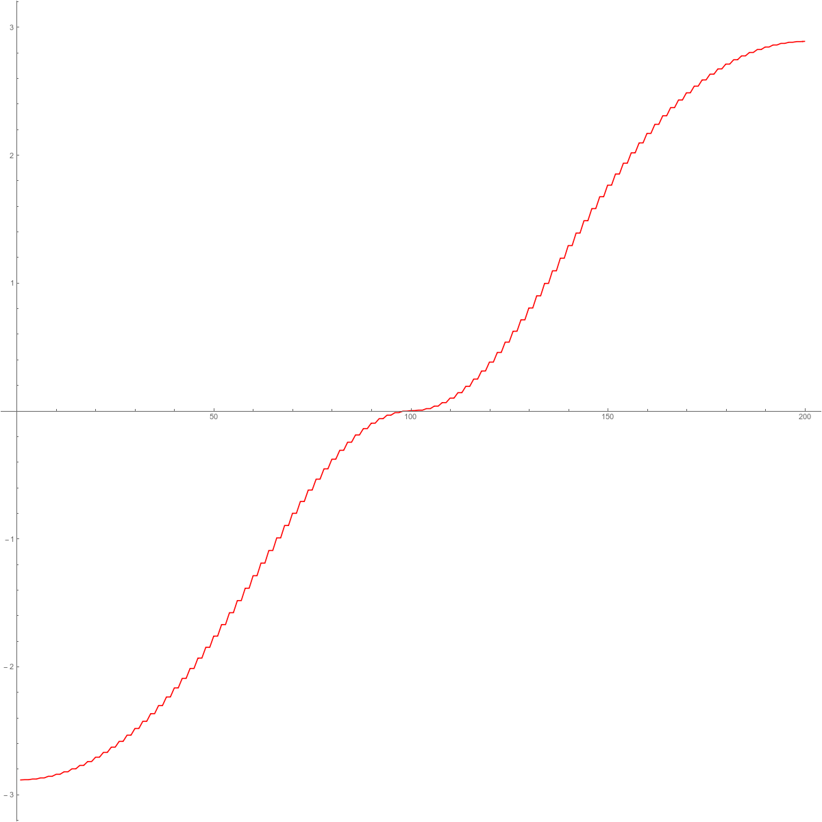
Lets look at a few graphs. In each case, if $\lambda_k$ are the eigenvalues, we look at the function $f(x) = \lambda_{[n x]}$, (where as usual the notation $[q]$ is the floor function, giving the largest integer smaller or equal to q). The inverse of this function is the integrated density of states (the cumulative distribution function for the probabilist). In the second graph we see the mass gap for the connection Laplacian. This is the main source for the excitement about the connection Laplacian. The fact that L is invertible even in the Barycentric limit makes the story not only exciting. It renders much of the matheatics very simple. The last picture illustrates the spectral symmetry $\sigma(L)=1/\sigma(L)$ for the connection Laplacian of a one-dimensional complex. We will just see that we can still compute this limiting graph explicitly like in the Hodge case.
|
|
|
|
| The eigenvalues of $H=D^2$. | The eigenvalues of $L$. | The eigenvalues of $L^2$. | The eigenvalues of $\log(L^2)$. |
The Hydrogen operator
In this paper we looked at the operator $Hydro=L-L^{-1}$. We especially looked at a Dehn-Sommerville functional $tr(Hydro)$. It was interesting for us because it is $f'(0)-f'(-1)$ for a generating function of a f-vector and also because it is the sum of the Euler characteristic of the unit spheres of the Barycentric refinement of G. It was called the Hydrogen operator because $-\Delta + 1/|x-y|$ is the quantum mechanical energy Hamiltonian of the Hydrogen atom and the inverse of $\Delta$ in $R^3$ has the kernel $g(x,y)=1/|x-y|$. It is natural to look also here for the operator $L-L^{-1}$. But it does not seem to help much: we get
$$ L-L^{-1} = \left[
\begin{array}{cccccccccccccccc}
2 & 1 & 0 & 0 & 0 & 0 & 0 & 1 & 0 & 0 & 0 & 0 & 0 & 0 & 0 & 0 \\
1 & 2 & 1 & 0 & 0 & 0 & 0 & 0 & 0 & 0 & 0 & 0 & 0 & 0 & 0 & 0 \\
0 & 1 & 2 & 1 & 0 & 0 & 0 & 0 & 0 & 0 & 0 & 0 & 0 & 0 & 0 & 0 \\
0 & 0 & 1 & 2 & 1 & 0 & 0 & 0 & 0 & 0 & 0 & 0 & 0 & 0 & 0 & 0 \\
0 & 0 & 0 & 1 & 2 & 1 & 0 & 0 & 0 & 0 & 0 & 0 & 0 & 0 & 0 & 0 \\
0 & 0 & 0 & 0 & 1 & 2 & 1 & 0 & 0 & 0 & 0 & 0 & 0 & 0 & 0 & 0 \\
0 & 0 & 0 & 0 & 0 & 1 & 2 & 1 & 0 & 0 & 0 & 0 & 0 & 0 & 0 & 0 \\
1 & 0 & 0 & 0 & 0 & 0 & 1 & 2 & 0 & 0 & 0 & 0 & 0 & 0 & 0 & 0 \\
0 & 0 & 0 & 0 & 0 & 0 & 0 & 0 & 2 & 1 & 1 & 0 & 0 & 0 & 0 & 0 \\
0 & 0 & 0 & 0 & 0 & 0 & 0 & 0 & 1 & 2 & 0 & 0 & 0 & 0 & 0 & 1 \\
0 & 0 & 0 & 0 & 0 & 0 & 0 & 0 & 1 & 0 & 2 & 1 & 0 & 0 & 0 & 0 \\
0 & 0 & 0 & 0 & 0 & 0 & 0 & 0 & 0 & 0 & 1 & 2 & 1 & 0 & 0 & 0 \\
0 & 0 & 0 & 0 & 0 & 0 & 0 & 0 & 0 & 0 & 0 & 1 & 2 & 1 & 0 & 0 \\
0 & 0 & 0 & 0 & 0 & 0 & 0 & 0 & 0 & 0 & 0 & 0 & 1 & 2 & 1 & 0 \\
0 & 0 & 0 & 0 & 0 & 0 & 0 & 0 & 0 & 0 & 0 & 0 & 0 & 1 & 2 & 1 \\
0 & 0 & 0 & 0 & 0 & 0 & 0 & 0 & 0 & 1 & 0 & 0 & 0 & 0 & 1 & 2 \\
\end{array}
\right] \; $$
But this might just look not good because the simplices are not aligned well. A matrix always depends on the chosen basis. A more natural ordering of the simplices is $G = \{ 1,12,2,23,3,34,…,7,78,8,81 \}.$ Bingo! Now the Hydrogen operator is nice
$$ Hydro = \left[
\begin{array}{cccccccccccccccc}
2 & 0 & 1 & 0 & 0 & 0 & 0 & 0 & 0 & 0 & 0 & 0 & 0 & 0 & 1 & 0 \\
0 & 2 & 0 & 1 & 0 & 0 & 0 & 0 & 0 & 0 & 0 & 0 & 0 & 0 & 0 & 1 \\
1 & 0 & 2 & 0 & 1 & 0 & 0 & 0 & 0 & 0 & 0 & 0 & 0 & 0 & 0 & 0 \\
0 & 1 & 0 & 2 & 0 & 1 & 0 & 0 & 0 & 0 & 0 & 0 & 0 & 0 & 0 & 0 \\
0 & 0 & 1 & 0 & 2 & 0 & 1 & 0 & 0 & 0 & 0 & 0 & 0 & 0 & 0 & 0 \\
0 & 0 & 0 & 1 & 0 & 2 & 0 & 1 & 0 & 0 & 0 & 0 & 0 & 0 & 0 & 0 \\
0 & 0 & 0 & 0 & 1 & 0 & 2 & 0 & 1 & 0 & 0 & 0 & 0 & 0 & 0 & 0 \\
0 & 0 & 0 & 0 & 0 & 1 & 0 & 2 & 0 & 1 & 0 & 0 & 0 & 0 & 0 & 0 \\
0 & 0 & 0 & 0 & 0 & 0 & 1 & 0 & 2 & 0 & 1 & 0 & 0 & 0 & 0 & 0 \\
0 & 0 & 0 & 0 & 0 & 0 & 0 & 1 & 0 & 2 & 0 & 1 & 0 & 0 & 0 & 0 \\
0 & 0 & 0 & 0 & 0 & 0 & 0 & 0 & 1 & 0 & 2 & 0 & 1 & 0 & 0 & 0 \\
0 & 0 & 0 & 0 & 0 & 0 & 0 & 0 & 0 & 1 & 0 & 2 & 0 & 1 & 0 & 0 \\
0 & 0 & 0 & 0 & 0 & 0 & 0 & 0 & 0 & 0 & 1 & 0 & 2 & 0 & 1 & 0 \\
0 & 0 & 0 & 0 & 0 & 0 & 0 & 0 & 0 & 0 & 0 & 1 & 0 & 2 & 0 & 1 \\
1 & 0 & 0 & 0 & 0 & 0 & 0 & 0 & 0 & 0 & 0 & 0 & 1 & 0 & 2 & 0 \\
0 & 1 & 0 & 0 & 0 & 0 & 0 & 0 & 0 & 0 & 0 & 0 & 0 & 1 & 0 & 2 \\
\end{array}
\right] \; . $$
We can now use Fourier to get the spectrum $\mu_k$ of Hydro and from that get the eigenvalues of $L$ as $f^{\pm}(\mu_k)$, where $f^{\pm}(y) = (y \pm \sqrt{4+y^2})/2$. We see that the density of states of the connection Laplacian is still a natural equilibrium measure on a union of two intervals. It is just conformally transplanted by a transformation which symmetrizes the spectrum.
More about the limiting Zeta function
[Update: January 8 2018:] I spent the last days writing and also looked more on the structure of the limiting zeta function. I finally managed to get an explicit expression
$$ \zeta(it)=_4F_3\left(\frac{1}{4},\frac{3}{4},-it,it;\frac{1}{2},\frac{1}{2},1;-4\right) $$
in terms of a hypergeometric series (this is a series $\sum_n c_n$ where successive $c_{n+1}/c_n$ are rational functions. Unfortunately, this does not help much as the actual series as given only makes sense through analytic continuation. Series of type $_4F_3$ have a radius of convergence of $1$ and the series is evaluated at $-4$. How was this obtained? Mathematica needed a lot of help here and to be forced to do some subsitutions and nonlinear substitutions u=z-1/z played an important role (no surprise as this is how the explicit expression was obtained after all). I also managed to write the function as a cos-transform of a function supported on the interval [0,log(2+\sqrt{5}]$:
h[y_]:=Sqrt[Cosh[y] Coth[y]/(2-Sinh[y])];
H[t_]:=NI[Cos[t*y]*h[y],{y,0,Log[2+Sqrt[5]]}]/Pi;  (* Cos Transform *)
And here is how Mathematica writes the function in terms of the hypergeometric series:
X[t_]:=HypergeometricPFQ[{1/4,3/4,-I t/2,I t/2},{1/2,1/2,1},-4];
While this function obviously is very nice and regular and has only real roots, we have not found a reference yet which tells something about the roots. There is a nice book of W.N. Bailey on Generalized Hypergeometric Series (from 1964) but the focus there (as at most other places) is to look at hypergeometric series as a function of z (the last entry). in our case, the variable s (rsp. it) appears in the Pochhammer expressions. Also, most seems to be known about the series of the type $_2F_1$ (the classical hypergeometric series) or then when evaluated at z=1. A prototype of the later is $F(a,b;c;1)=\Gamma(c)\Gamma(c-a-b)/(\Gamma(c-a) \Gamma(c-b))$, an expression due to Gauss. In our case, $z=-4$, the hypergeometric series does not even converge and Mathematica obviously uses some analytic continuation here. It is in such situations a big disadvantage to work with a computer algebra system which is opaque in the sense that a lot of knowledge is hidden and not documented. ]
About product spaces
[Update: January 9, 2018] I would like to share an other picture added yesterday to the article. It deals with the product of simplicial complexes G x H. this is the product in the strong ring of simplicial complexes. It is a very simple product: remember that G and H are just finite sets of sets. Now, we can build the set theoretical product set $G \times H$. This is no simplicial complex any more but it has a geometric structure. Its Barycentric refinement is the Whitney complex of a graph. I had looked at this product in the Kuenneth paper but that product $(G,H) \to (G \times H)_1$ is not associative. It is better to chill out therefore and drop the requirement of dealing with simplicial complexes. One can just generate a new ring of geometric objects and that is what the “strong ring is about”. We are very familiar with that construct. If we think of a square for example, then we think about it as a two dimensional product of two intervals. It is not a simplicial complex however as the two dimensional cell is not a triangle. But we think of it as a 2-dimensional CW complex, where one starts with the empty space, adds 4 zero-dimensional cells (glued to the empty complex, which is the -1 dimensional sphere), then glues in 4 one dimensional cells along zero dimensional spheres (pairs of disjoint zero dimensional points), then at the very end, a 2-cell has been glued in along the circle $C_4$. This is where we deviated from the construction of a simplicial complex as we glued along a sphere which is not a hypersceleton of a simplex) So, we think of the product space as a CW complex. But we can look at the connection Laplacian $L_{G \times H}$ of the product $G \times H$ without thinking about CW constructions. The matrix entry L( (x,y),(u,v) ) is $1$ if both $x \cap u \neq \emptyset$ and $y \cap v \neq \emptyset$. Otherwise, if one of the links is not present, we put $L( (x,y),(u,v)) = 0$.
Now, we have noticed and proven in the strong ring paper that
| The spectrum of $L_{G \times H}$ is the product of the spectrum of $L_G$ and $L_H$. |
This is unlike the Hodge Laplacian H (which is a matrix on the same Hilbert space), where the spectrum adds up (as for the classical Hodge Laplacians). The reason why this is true is because the product connection Laplacian is the tensor product of the individual Laplacians. There is a bit of a pickle here as the tensor product of matrices is not commutative but the product of simplicial complexes is. But this is just because we have to commit to a basis. The two tensor products are similar. See Lemma 9 and corollary 4 in the strong ring paper). But now we have the following nice corollary
| The zeta function $\zeta_{G \times H}$ is the product of the zeta functions $\zeta_G$ and $\zeta_H$. |
which implies for the roots
| The roots of the zeta function $\zeta_{G \times H}$ is the union of the roots of the zeta functions $\zeta_G$ and $\zeta_H$. |
Proof. $\zeta_{G \times H}(s) = \sum_{\lambda,\mu} (\lambda \mu)^{-s}$ = $\sum_{\lambda} \sum_{\mu} \lambda^{-s} \mu^{-s} = (\sum_{\lambda} \lambda^{-s})(\sum_{\mu} \mu^{-s}) = \zeta_G(s) \zeta_H(s)$.
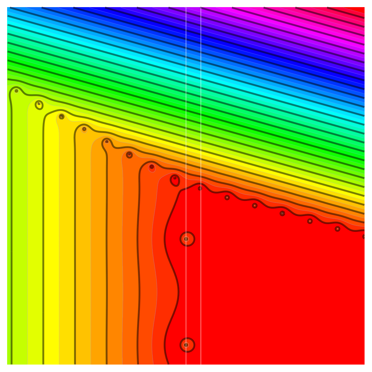
So, and here is the picture. We see first the picture of the zeta function of the interval complex $G=K_2$ (which is a one dimensional complex which has the functional equation symmetry) then the zeta function of the triangle $H=K_3$ (which does not have the functional equation symmetry). The product $G \times H$ can be thought of a solid cylinder. It is a three dimensional CW complex and not a simplicial complex. We actually noted in the “strong ring paper” that in the strong ring, the simplicial complexes are the “multiplicative primes”. (The additive primes are the topological connected components of a space). The solid cylinder is not a prime as it can be written as a product of two primes, the interval and the disk. You see clearly in the picture how the roots have unionized. This is what happens when you take the product of two analytic functions.
Well and here are the connection Laplacians for $G=\{\{1,2\},\{1\},\{2\}\}$
$$ L_G=\left[
\begin{array}{ccc}
1 & 1 & 1 \\
1 & 1 & 0 \\
1 & 0 & 1 \\
\end{array}
\right] $$
with eigenvalues $\left\{1+\sqrt{2},1,1-\sqrt{2}\right\}=\{2.41421,1.,-0.414214\}$. For the second complex $H=\{\{1,2,3\},\{1\},\{2\},\{3\},\{1,2\},\{1,3\},\{2,3\}\}$ the connection Laplacian is
$$
L_H=\left[
\begin{array}{ccccccc}
1 & 1 & 1 & 1 & 1 & 1 & 1 \\
1 & 1 & 0 & 0 & 1 & 1 & 0 \\
1 & 0 & 1 & 0 & 1 & 0 & 1 \\
1 & 0 & 0 & 1 & 0 & 1 & 1 \\
1 & 1 & 1 & 0 & 1 & 1 & 1 \\
1 & 1 & 0 & 1 & 1 & 1 & 1 \\
1 & 0 & 1 & 1 & 1 & 1 & 1 \\
\end{array}
\right]
$$
which has the eigenvalues $\{5.5114,1.61803,1.61803,-0.752518,-0.618034,-0.618034,0.241113\}$. The product space $G \times H$ is a set of sets but not a simplicial complex:
$$
\left(
\begin{array}{cc}
\{1,2\} & \{1,2,3\} \\
\{1,2\} & \{1\} \\
\{1,2\} & \{2\} \\
\{1,2\} & \{3\} \\
\{1,2\} & \{1,2\} \\
\{1,2\} & \{1,3\} \\
\{1,2\} & \{2,3\} \\
\{1\} & \{1,2,3\} \\
\{1\} & \{1\} \\
\{1\} & \{2\} \\
\{1\} & \{3\} \\
\{1\} & \{1,2\} \\
\{1\} & \{1,3\} \\
\{1\} & \{2,3\} \\
\{2\} & \{1,2,3\} \\
\{2\} & \{1\} \\
\{2\} & \{2\} \\
\{2\} & \{3\} \\
\{2\} & \{1,2\} \\
\{2\} & \{1,3\} \\
\{2\} & \{2,3\} \\
\end{array}
\right) .
$$
Using this basis, we get the connection Laplacian of the product:
$$
L_{G \times H} \left[
\begin{array}{ccccccccccccccccccccc}
1 & 1 & 1 & 1 & 1 & 1 & 1 & 1 & 1 & 1 & 1 & 1 & 1 & 1 & 1 & 1 & 1 & 1 & 1 & 1 & 1 \\
1 & 1 & 0 & 0 & 1 & 1 & 0 & 1 & 1 & 0 & 0 & 1 & 1 & 0 & 1 & 1 & 0 & 0 & 1 & 1 & 0 \\
1 & 0 & 1 & 0 & 1 & 0 & 1 & 1 & 0 & 1 & 0 & 1 & 0 & 1 & 1 & 0 & 1 & 0 & 1 & 0 & 1 \\
1 & 0 & 0 & 1 & 0 & 1 & 1 & 1 & 0 & 0 & 1 & 0 & 1 & 1 & 1 & 0 & 0 & 1 & 0 & 1 & 1 \\
1 & 1 & 1 & 0 & 1 & 1 & 1 & 1 & 1 & 1 & 0 & 1 & 1 & 1 & 1 & 1 & 1 & 0 & 1 & 1 & 1 \\
1 & 1 & 0 & 1 & 1 & 1 & 1 & 1 & 1 & 0 & 1 & 1 & 1 & 1 & 1 & 1 & 0 & 1 & 1 & 1 & 1 \\
1 & 0 & 1 & 1 & 1 & 1 & 1 & 1 & 0 & 1 & 1 & 1 & 1 & 1 & 1 & 0 & 1 & 1 & 1 & 1 & 1 \\
1 & 1 & 1 & 1 & 1 & 1 & 1 & 1 & 1 & 1 & 1 & 1 & 1 & 1 & 0 & 0 & 0 & 0 & 0 & 0 & 0 \\
1 & 1 & 0 & 0 & 1 & 1 & 0 & 1 & 1 & 0 & 0 & 1 & 1 & 0 & 0 & 0 & 0 & 0 & 0 & 0 & 0 \\
1 & 0 & 1 & 0 & 1 & 0 & 1 & 1 & 0 & 1 & 0 & 1 & 0 & 1 & 0 & 0 & 0 & 0 & 0 & 0 & 0 \\
1 & 0 & 0 & 1 & 0 & 1 & 1 & 1 & 0 & 0 & 1 & 0 & 1 & 1 & 0 & 0 & 0 & 0 & 0 & 0 & 0 \\
1 & 1 & 1 & 0 & 1 & 1 & 1 & 1 & 1 & 1 & 0 & 1 & 1 & 1 & 0 & 0 & 0 & 0 & 0 & 0 & 0 \\
1 & 1 & 0 & 1 & 1 & 1 & 1 & 1 & 1 & 0 & 1 & 1 & 1 & 1 & 0 & 0 & 0 & 0 & 0 & 0 & 0 \\
1 & 0 & 1 & 1 & 1 & 1 & 1 & 1 & 0 & 1 & 1 & 1 & 1 & 1 & 0 & 0 & 0 & 0 & 0 & 0 & 0 \\
1 & 1 & 1 & 1 & 1 & 1 & 1 & 0 & 0 & 0 & 0 & 0 & 0 & 0 & 1 & 1 & 1 & 1 & 1 & 1 & 1 \\
1 & 1 & 0 & 0 & 1 & 1 & 0 & 0 & 0 & 0 & 0 & 0 & 0 & 0 & 1 & 1 & 0 & 0 & 1 & 1 & 0 \\
1 & 0 & 1 & 0 & 1 & 0 & 1 & 0 & 0 & 0 & 0 & 0 & 0 & 0 & 1 & 0 & 1 & 0 & 1 & 0 & 1 \\
1 & 0 & 0 & 1 & 0 & 1 & 1 & 0 & 0 & 0 & 0 & 0 & 0 & 0 & 1 & 0 & 0 & 1 & 0 & 1 & 1 \\
1 & 1 & 1 & 0 & 1 & 1 & 1 & 0 & 0 & 0 & 0 & 0 & 0 & 0 & 1 & 1 & 1 & 0 & 1 & 1 & 1 \\
1 & 1 & 0 & 1 & 1 & 1 & 1 & 0 & 0 & 0 & 0 & 0 & 0 & 0 & 1 & 1 & 0 & 1 & 1 & 1 & 1 \\
1 & 0 & 1 & 1 & 1 & 1 & 1 & 0 & 0 & 0 & 0 & 0 & 0 & 0 & 1 & 0 & 1 & 1 & 1 & 1 & 1 \\
\end{array}
\right]
$$
which has the eigenvalues $\{13.3057,5.5114,3.90628,3.90628,-2.2829$, $-1.81674,1.61803,1.61803,-1.49207,-1.49207$, $-0.752518,-0.670212,-0.670212$, $-0.618034,-0.618034,0.582099,0.311703,0.255998$, $0.255998,0.241113,-0.0998723\}$. This is the set of all products of the individual eigenvalues of the simplices in G and H. The largest eigenvalue for example, $13.3057$, is the product $2.41421*5.5114$ of the largest eigenvalues of $G$ and $H$.
The Friedli-Karlsson conjecture
In a nice recent paper of Fabien Friedli and Anders Karlsson, called “Spectral zeta functions of graphs and the Riemann zeta function in the critical strip”, the zeta function of the Kirchhoff Laplacian of circular graphs is studied in more detail. These authors (both from the university of Geneva) were obviously not aware of my paper on the zeta function of circular graphs and there is some overlap, but there is no question that their work is much nicer. (My paper was a bit of entertainment done in the summer of 2013 and was never submitted to a journal). I’m really happy however that the subject has the attention it deserves. But most importantly, there is a big surprise:
There is a conjecture of Friedli and Karlsson about zeta functions of circular graphs which is equivalent to the Riemann zeta function.
I had suspected then that any connection between the finite dimensional Riemann zeta functions and the continuum would be very difficult and technical. It appears however that it boils down to a question on how fast the approximation of a Riemann sum of a concrete one-dimensional function is to an integral. Before we start with stating their conjecture, let us make a remark why there is a discrepancy between notations.
[Remark (can easily be scipped) There is a bit of a discrepancy in whether to take s or 2s or s/2 in the definitions. In my paper, I used the spectral zeta function without dividing s by 2, which had the effect that the roots accumulated on the line Re(s)=1 and not the usual $Re(s)=1/2$.The reason of the discrepancy had been explained above: if one takes the zeta function of the Laplacian $-d/dx^2$ on the circle $T$ which has the eigenvalues $\lambda=n^2$ with eigenfunctions $\cos(nx), \sin(nx)$ then $\sum_n \lambda^{-s}$ is the spectral zeta function of the Laplacian and $\sum_n \lambda^{-s/2}$ is the spectral zeta function of the Dirac operator $D=i d/dx$. This shows that any result about $Re(s)=1$ for the Laplacian corresponds to the case $Re(s)=1/2$ for the Dirac operator. As also explained above, in the Dirac case, one disregards the “anti matter” part (negative eigenvalues) as there would be ambiguity of choosing a square root for every eigenvalue. One therefore takes the normalized zeta function $\sum_n \lambda^{-s/2}$. This silly looking gymnastics explains the factor 2 discrepancy in the various papers. It is not a problem but it is important that one realizes that this is not just convenience but that the factor 2 has come in naturally to avoid negative spectrum and still work with the Dirac spectrum. I call this the normalized Zeta function of a self adjoint matrix $A$: it is defined as $\sum_{n} (\lambda^2)^{s/2}$ which is not the same thing in complex analysis than $\sum_{n} \lambda^s$. Taking in the exponent half but square the negative numbers avoids serious confusions, even for (smart) computer algebra systems. Here are pictures of the zeta function for the non-normalized zeta function of $K_2= \{ \{1,2\},\{1\},\{2\} \}$ and then the normalized zeta function:
|
|
You see clearly that we have a “mess” on the left picture while the right picture shows the spectral symmetry (functional equation) we have talked about a lot before in this blog entry. The connection Laplacian is the matrix
$$ L = \left[
\begin{array}{ccc}
1 & 1 & 1 \\
1 & 1 & 0 \\
1 & 0 & 1 \\
\end{array}
\right] $$
which has the eigenvalues $ \left\{1+\sqrt{2},1,1-\sqrt{2}\right\}$. The non-normalized zeta function is $\zeta_L(s) = (-0.414214)^{-s}+1.^{-s}+2.41421^{-s}$. The normalized zeta function is $\zeta_{L^2}(s/2) = 0.171573^{-s/2}+1.^{-s/2}+5.82843^{-s/2}$. Because one is tired to write all these $s/2$ all the time, I had opted in my 2013 paper to use the double s, leading to Re(s)=1 rather than Re(s)=1/2. Also here in the connection story, I don’t bother taking s rather than s/2. It does matter very little here as in the connection case the functional equation has the y axes as an axes of symmetry. End of Remark]
Friedli and Karsson look at the spectral zeta function $\zeta_n(s) = 4^{-s} \sum_{k=1}^n \sin^{2s}(\pi k/n)$ of circular graphs, (which is $\zeta_n(2s)$ in (2) of my paper) and call $\zeta_Z(s)=\frac{4^{-s} \Gamma \left(\frac{1}{2}-s\right)}{\sqrt{\pi } \Gamma (1-s)}$
the spectral function of the $Z$. This is the function $c(2s)$ on page 6 of my paper. Here is already something, I did not know:
the entire completion $\xi_Z(s) = 2^s \cos(\pi s/2) \zeta_z(s/2)$ satisfies the functional equation $\xi_Z(s)=\xi_Z(1-s)$ (see their Theorem 0.2).
Theorem 0.3 in their paper is close to Theorem 10 and Proposition 9 in my case. It deals with the asymptotics. Now here is the surprise: on page 605 of \cite{FriedliKarsson} there is a statement which shows that $\zeta_n$ indeed has some relation with the Riemann zeta function. Friedli-Karsson introduce
$$ h_n(s)=(4\pi)^{s/2} \Gamma(s/2) n^{-s}(\zeta_n(s/2)-n\zeta_Z(s/2) \; . $$
and show that
$$ \lim_{n \to \infty} |h_n(1-s)/h_n(s)|=1 $$
in the critical strip Re(s) in [0,1] is equivalent to the Riemann hypothesis.
We can rephrase this a bit as we clearly see that the factors $s/2$ appears everywhere:
| [Friedli-Karsson conjecture (equivalent to Riemann hypothesis)] The function $$ H_n(s)=(4 \pi)^s \Gamma(s) n^{1-2s} [ \frac{\zeta_n(s)}{n} – \zeta(s) ] $$ satisfy $\lim_{n \to \infty} |H_n(2-s)/H_n(s)|=1$ for all s with real part in [0,2]. |
Why did we take out the additional factor $n$ in the reformulation? Because now the part in the bracket $\zeta_n(s)/n – \zeta(s)$ is the error of a Riemann sum approximation of the function $g(x) = 4 \sin(\pi x)^{-s}$. This function is parametrized by the parameter s, but for each fixed x, we deal with a function on the interval $[0,1]$. The limiting case is the integral, the circular approximation case is the Riemann sum.
Well, this hits right at the heart of where I had been battling stuff also when dealing with the Birkhoff sum of the cot function, where I give an example of a Birkhoff sum over an ergodic translation where one can give an exact formula for the limiting self similar growth. (That paper had been motivated and out-grown from work with Folkert Tangerman on Birkhoff sums for the golden rotation). So, what is the idea of estimating the difference between a Riemann sum and the integral? When learning single variable calculus one gets introduced to the mean value theorem. This motivates to look at the Rolle point of a function f. It is a point which could be taken as an evaluation point rather than integrating over the interval. Given an interval $[x_0-a,x_0+a]$ one looks for the solution $x$ of the equation $f(x_0+a)-f(x_0-a) – 2a f'(x) = 0$. The mean value theorem shows that there exists a solution in [-a,a]. I defined the Rolle point as the point closest to $x_0$ solving this equation and which is to the right of $x_0$ (if there should be two solutions in equal distance closest). I have given the formula $f(0) + (\frac{f'(0) f”'(0) }{12 f”(0)^2}) f”(0) a^2 + O(a^4)$ which led to the notion of a K-derivative
$$ K_g(x) = \frac{g'(x) g”'(x)}{g”(x)^2} \; . $$
It has similar features to the Schwarzian derivative
$$ S_g(x) = \frac{g”'(x)}{g'(x)} – \frac{3}{2} \frac{g”(x)}{g'(x))^2} \; $$
which is important in the theory of one-dimensional maps (a bit more close where I come from as Oscar Lanford, who was one of the great experts of the dynamics of one dimensional maps, taught us about that also in a 2 semester intro course about dynamical systems). Why the letter $K$? Well, The Schwarzian derivative was introduced by Hermann Schwarz [who is the Schwarz from the Cauchy-Schwarz inequality], now figure … (;-))
Here is something right from my 2013 paper: as the following examples show, they lead to similarly simple expressions, if we evaluate it for some basic functions:
| $g$ | Schwarzian $S_g$ | K-Derivative $K_g$ |
| $\cot(kx)$ | $2k^2$ | $1+\sec^2(kx)/2$ |
| $\sin(x)$ | $-1-3 \tan^2(x)/2$ | $-\cot^2(x)$ |
| $x^s$ | $(1-s^2)/(2x^2)$ | $(s-2)/(s-1)$ |
| $1/x$ | $0$ | $3/2$ |
| $\log(x)$ | $0$ | $2$ |
| $\exp(x)$ | $-1/2$ | $1$ |
| $\log(\sin(x))$ | $\frac{1}{2}\csc^2(x)[4-3 \sec ^2(x)]$ | $2\cos^2(x)$ |
| $\frac{ax+b}{cx+d}$ | $0$ | $3/2$ |
Both notions involve the first three derivatives of $g$. [The Latex Plugin in WordPress unfortunately simplifies ” so that the expressions look awkward.] The $K$-derivative is invariant under linear transformations $K_{ag+b}(y) = K_g(y)$ and a constant for $g(x)=x^n, n \neq 0,1$ or $g(x)=\log(x)$ or $g(x)=\exp(x)$.
Note that while the Schwarzian derivative is invariant under fractional linear transformations
$$ S_{(ag+b)/(cg+d)}(y) = S_g(y) \; , $$
the K-derivative is invariant under linear transformations only. It vanishes on quadratic functions. An important example for the zeta story is the function $g(x) = 1/\sin^s(x)$ for which
$$ K_g(x) = \frac{2 \cos^2(x) \left(s^2 \cos (2 x)+s^2+6 s+4\right)}{(s \cos (2 x)+s+2)^2} \; $$
is bounded if $s>-1$. Also all even derivatives are finite.