Quantum Calculus

Euler and Fredholm

The following picture illustrates the Euler and Fredholm theme in the special case of the prime graphs introduced in the Counting and Cohomology paper. The story there only dealt with the Euler characteristic, an additive valuation (in the sense of Klain and Rota). Since then, the work on the Fredholm …

The Unimodularity Theorem for CW Complexes

The unimodularity theorem equates a fredholm determinant with a product of indices. It originally was formulated for graphs or simplicial complexes. It turns out to be valid for more general structures, generalized cellular complexes. While for discrete CW complexes, the fredholm determinant is 1 or -1, in general it can now take more general values but the structures are also more strange: in the continuum much more general than CW complexes as the attached cells do not need to be bound by spheres but can be rather arbitrary.

The Kustaanheimo prime

Paul Kustaanheimo (1924-1997) was a Finnish astronomer and mathematician. In celestial mechanics, his name is associated with the Kustaanheimo-Stiefel transform or shortly KS transform which allows to regularize the Kepler problem using Clifford algebras. In this elegant picture, the motion of the two bodies becomes a rotation in three dimensions …

Counting and Cohomology

There are various cohomologies for finite simplicial complexes. If the complex is the Whitney complex of a finite simple graph then many major results from Riemannian manifolds have discrete analogues. Simplicial cohomology has been constructed by Poincaré already for simplicial complexes. Since the Barycentric refinement of any abstract finite simplicial complex is always the Whitney complex of a finite simple graph, there is no loss of generality to study graphs instead of abstract simplicial complexes. This has many advantages, one of them is that graphs are intuitive, an other is that the data structure of graphs exists already in all higher order programming languages. A few lines of computer algebra system allow so to compute all cohomology groups. The matrices involved can however become large, so that alternative cohomologies are desired.

Interaction cohomology

[Update, March 20, 2018: see the ArXiv text. See also an update blog entry with some Mathematica code. More mathematica code can be obtained from the TeX Source of the ArXiv article.]. Classical calculus we teach in single and multi variable calculus courses has an elegant analogue on finite simple …

Wu Characteristic

Update: March 8, 2016: Handout for a mathtable talk on Wu characteristic. Gauss-Bonnet for multi-linear valuations deals with a number in discrete geometry. But since the number satisfies formulas which in the continuum need differential calculus, like curvature, the results can be seen in the light of quantum calculus. Here …

Exponential Function

We have seen that f'(x)=Df(x) = (f(x+h)-f(x))/h satisfies D[x]^n = n [x]^{n-1}.
We will often leave the constant $h$ out of the notation and use terminology like f'(x) = Df(x) for the “derivative”. It makes sense not to simplify [x]^n to $x^n$ since the algebra structure is different.

Define the exponential function as
exp(x) = \sum_{k=0}^{\infty} [x]^k/k!. It solves the equation Df=f. Because each of the approximating polynomials exp_n(x) = \sum_{k=0}^{n} [x]^k/k! is monotone and positive also exp(x) is monotone and positive for all x. The fixed point equation Df=f reads f(x+h) = f(x) + h f(x) = (1+h) f(x) so that for h=1/n we have f(x+1) = f(x+n h) = (1+h)^n f(x) = e_n f(x)
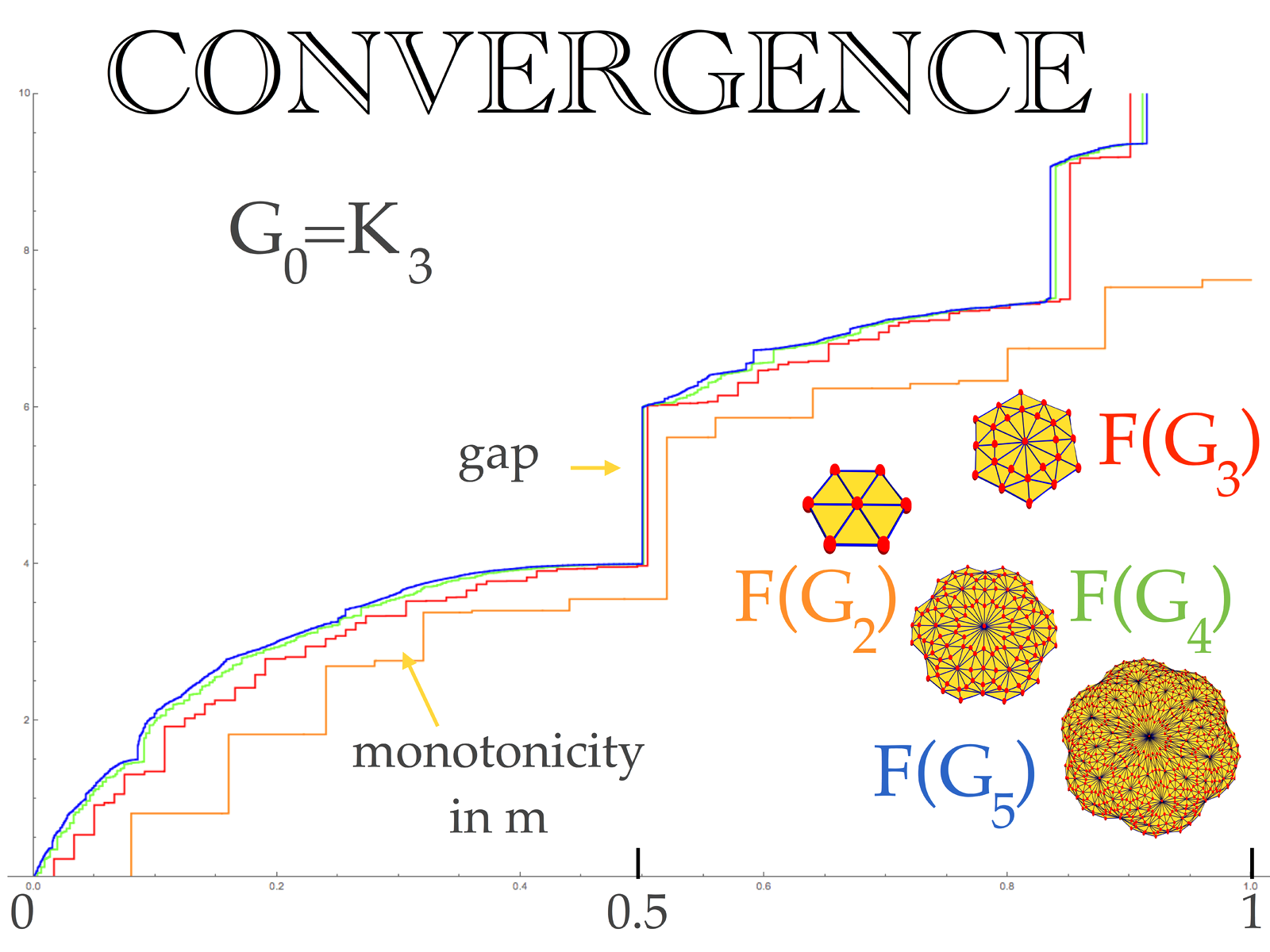
where $e_n \to e$. Because $n \to e_n$ is monotone, we see that the exponential function \exp(x) depends in a monotone manner on h and that for h \to 0 the graphs of $\exp(x)$ converge to the graph of \exp(x) as h \to 0.

Since the just defined exponential function is monotone, it can be inverted on the positive real axes. Its inverse is called \log(x). We can also define trigonometric functions by separating real and imaginary part of \exp(i x) = \cos(x) + i \sin(x). Since D\exp=\exp, these functions satisfy D\cos(x) = - \sin(x) and D\sin(x) = \cos(x) and are so both solutions to D^2 f = -f.

Fundamental Theorem

Let denote the discrete derivative of a continuous function f on the real line. In this post, I assume that all functions are continuous of have compact support. They are zero outside some large interval. No smoothness is required of course. Here is the simplest version of the fundamental theorem …

Critical points

Assume f is a continuous function of one real variable. Lets call a point p a critical point of f if Df(p)=0 where Df(x) = f(x+1)-f(x) is the discrete derivative of f. As in classical calculus, a point p is called a local maximum of f, if there exists an …